Download PDF
Brain atlas data as a ggplot2 layer
ggseg adds a single layer type to ggplot2. An atlas supplies the geometry, your data supplies the values.
library(ggseg)
library(ggplot2)

ggplot() +
  geom_brain(atlas = dk()) +
  theme_void()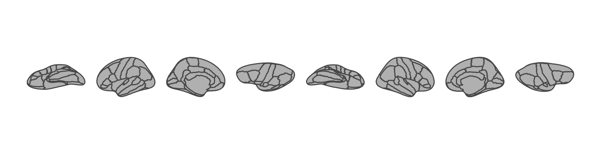
dk(), not dk.fill — see Atlas palettes.theme_void() removes the coordinate axes, which a brain plot has no use for.geom_brain(
mapping = aes(), data = NULL, atlas,
hemi = NULL, view = NULL,
position = position_brain(),
context = TRUE, fun = mean, ...
)| Atlas | Type | Covers |
|---|---|---|
dk() |
cortical | Desikan-Killiany, 35 regions per hemisphere |
aseg() |
subcortical | FreeSurfer automatic segmentation |
suit() |
cerebellar | SUIT cerebellar parcellation |
tracula() |
tract | TRACULA white-matter tracts |
Dozens more install from the ggsegverse r-universe — see the atlases and data structures sheet.
Accessors live in ggseg.formats, which ggseg loads but does not re-export:
library(ggseg.formats)

atlas_regions(dk())
atlas_labels(dk())
atlas_views(dk())
atlas_type(dk())Give ggplot() a data frame with a region or label column. geom_brain() joins it to the atlas, so you only name the regions you actually have.
scores <- data.frame(
  region = c("precentral", "insula", "fusiform"),
  score = c(1.2, -0.4, 0.8)
)

ggplot(scores) +
  geom_brain(atlas = dk(), aes(fill = score)) +
  scale_fill_gradient2() +
  theme_void()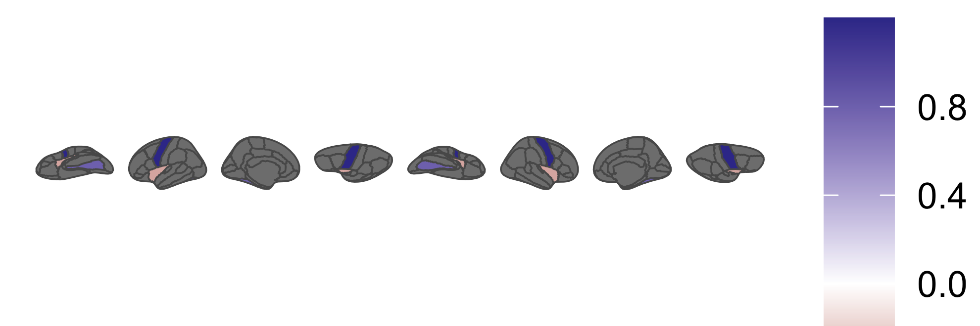
na.value — grey by default.label (lh_precentral) to colour one hemisphere only.fun = mean collapses several rows that share a region.brain_join(data, atlas, by = NULL) returns the merged table instead of a plot, when you want to inspect the join.Each facet gets a whole brain, so one plot can carry several contrasts.
long <- data.frame(
  region = rep(c("precentral", "insula", "fusiform"), 2),
  score = c(1.2, -0.4, 0.8, -1.1, 0.2, 1.6),
  session = rep(c("pre", "post"), each = 3)
)

ggplot(long) +
  geom_brain(atlas = dk(), aes(fill = score)) +
  facet_wrap(~session) +
theme_void()position_brain() decides where hemispheres and views sit. For cortical atlases, pass a formula of rows ~ columns.
ggplot() +
  geom_brain(
    atlas = dk(),
    position = position_brain(hemi ~ view)
  ) +
  theme_void()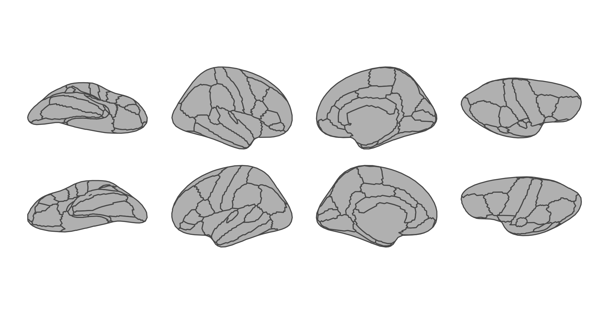
| Formula | Layout |
|---|---|
hemi ~ view |
hemispheres in rows, views in columns |
view ~ hemi |
views in rows, hemispheres in columns |
. ~ view + hemi |
a single row, every panel side by side |
hemi + view ~ . |
a single column, stacked |
# zoom each view onto its focus regions
position_brain(hemi ~ view, zoom = TRUE)

# zoom onto named regions, with 10% padding
position_brain(hemi ~ view, zoom = "insula", zoom_pad = 0.1)

# keep only these views, in this order
position_brain(views = c("lateral", "medial"))
Subcortical and tract atlases have slice views rather than hemispheres, so they take "horizontal", "vertical", nrow or ncol instead:
ggplot() +
  geom_brain(
    atlas = aseg(),
    position = position_brain("horizontal", nrow = 2)
  ) +
  theme_void()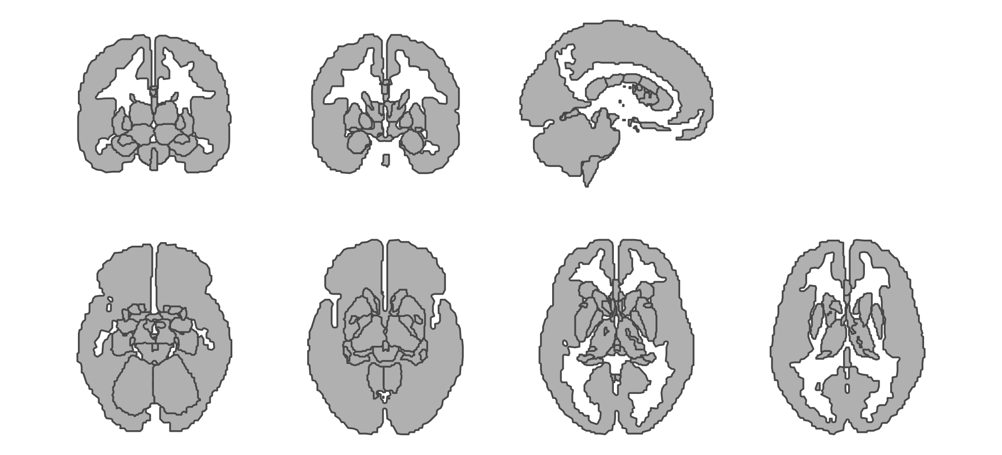
geom_brain(atlas = dk(), hemi = "left")
geom_brain(atlas = dk(), view = "lateral")
reposition_brain(data, position, ...) rearranges an already-joined atlas table, and coord_brain(ratio = 1) fixes the aspect ratio by hand.
Every atlas carries the colours its parcellation is normally drawn in. They are not applied automatically: map fill to label and hand the palette to scale_fill_manual().
ggplot() +
  geom_brain(
    atlas = dk(),
    aes(fill = label),
    show.legend = FALSE
  ) +
  scale_fill_manual(values = dk()$palette) +
  theme_void()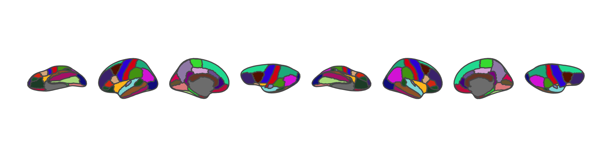
atlas_palette(dk()) returns the same named vector, and atlas_plot_palette(dk()) draws it as a swatch.
pal <- c(
  precentral = "#5e3c58",
  insula = "#a8c5cb"
)

ggplot() +
  geom_brain(
    atlas = dk(),
    aes(fill = region),
    show.legend = FALSE
  ) +
  scale_fill_brain_manual(pal, na.value = "grey90") +
  theme_void()
scale_fill_brain_manual(palette, na.value) — fill.scale_colour_brain_manual() / scale_color_brain_manual() — outlines.scale_brain_manual(palette, aesthetics) — both at once.For continuous values, use ggplot2’s own scales: scale_fill_viridis_c(), scale_fill_gradient2(), scale_fill_distiller().
Deprecated.
scale_fill_brain(),scale_brain()and the*_brain2()family are superseded. Usescale_fill_manual()withatlas$palette, or the*_brain_manual()functions above.
theme_brain(text.size = 12, text.family = "mono")
theme_darkbrain(text.size = 12)
theme_brain2(
  plot.background = "white",
  text.colour = "darkgrey"
)
theme_custombrain(
  plot.background = "white",
  text.colour = "darkgrey",
  text.size = 12
)
These keep the axes and style the surround; theme_darkbrain() is the one for dark slides. ggplot2::theme_void() is the right choice when you want nothing but the brain.
pos <- position_brain(hemi ~ view)

ggplot() +
  geom_brain(atlas = dk(), position = pos) +
  annotate_brain(dk(), position = pos, size = 1.5) +
  theme_void()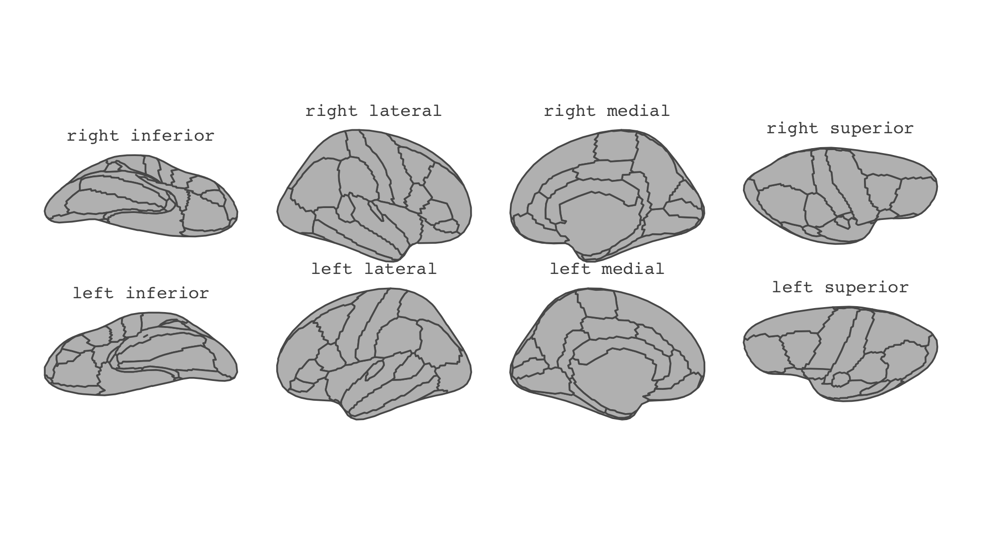
annotate_brain() writes the view name (“left lateral”) above each view. Pass it the same position you gave geom_brain().scale_labs_brain() and scale_continous_brain() put hemisphere and view labels on the axes in place of coordinates.geom_sf_text() on as_sf_atlas(dk()) if you need them.plot(dk())
brain_test_plot(
dk(),
position = position_brain(hemi ~ view)
)Both draw every region in its palette colour — the quickest way to see whether a new or edited atlas renders.
dk is a function; dk() is the atlas. The missing parentheses are the most common error.fill mapping is grey by design, not broken.setdiff(data$region, atlas_regions(dk())).context = FALSE drops the greyed-out surrounding structures that subcortical atlases draw for anatomical context.geom_brain_sf() and position_brain_sf() are deprecated; geom_brain() is the polygon default, and as_sf_atlas() gives you sf geometry for geom_sf().https://ggsegverse.github.io — ecosystem documentationvignette("ggseg") — longer worked exampleshttps://github.com/ggsegverse — source and issues