3D brain plotting with ggseg3d :: Cheatsheet

Interactive brain surfaces as an htmlwidget

ggseg3d(), cameras, surfaces, widget options and Shiny bindings.

Author

Athanasia Monika Mowinckel

Download PDF

Plotting

A brain in three dimensions

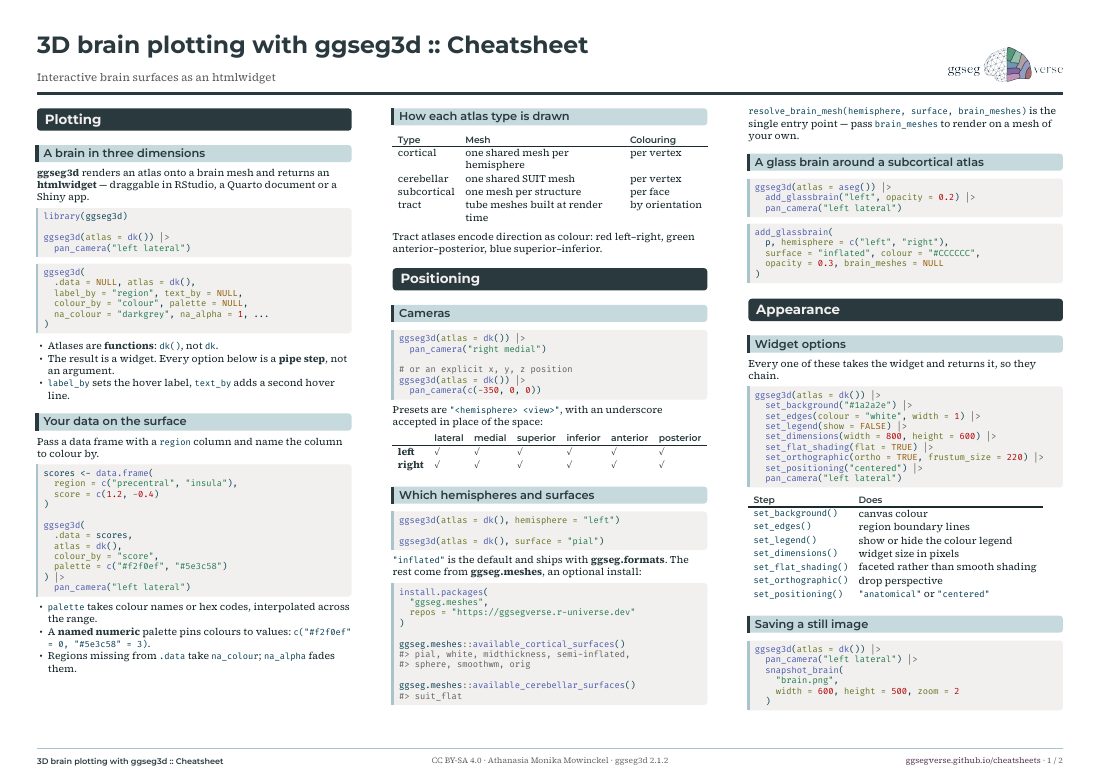
ggseg3d renders an atlas onto a brain mesh and returns an htmlwidget — draggable in RStudio, a Quarto document or a Shiny app.

library(ggseg3d)

ggseg3d(atlas = dk()) |>
  pan_camera("left lateral")

ggseg3d(
  .data = NULL, atlas = dk(),
  label_by = "region", text_by = NULL,
  colour_by = "colour", palette = NULL,
  na_colour = "darkgrey", na_alpha = 1, ...
)

Atlases are functions: dk(), not dk.
The result is a widget. Every option below is a pipe step, not an argument.
label_by sets the hover label, text_by adds a second hover line.

Your data on the surface

Pass a data frame with a region column and name the column to colour by.

scores <- data.frame(
  region = c("precentral", "insula"),
  score = c(1.2, -0.4)
)

ggseg3d(
  .data = scores,
  atlas = dk(),
  colour_by = "score",
  palette = c("#f2f0ef", "#5e3c58")
) |>
  pan_camera("left lateral")

palette takes colour names or hex codes, interpolated across the range.
A named numeric palette pins colours to values: c("#f2f0ef" = 0, "#5e3c58" = 3).
Regions missing from .data take na_colour; na_alpha fades them.

How each atlas type is drawn

Type	Mesh	Colouring
cortical	one shared mesh per hemisphere	per vertex
cerebellar	one shared SUIT mesh	per vertex
subcortical	one mesh per structure	per face
tract	tube meshes built at render time	by orientation

Tract atlases encode direction as colour: red left–right, green anterior–posterior, blue superior–inferior.

Positioning

Cameras

ggseg3d(atlas = dk()) |>
  pan_camera("right medial")

# or an explicit x, y, z position
ggseg3d(atlas = dk()) |>
  pan_camera(c(-350, 0, 0))

Presets are "<hemisphere> <view>", with an underscore accepted in place of the space:

	lateral	medial	superior	inferior	anterior	posterior
left	✓	✓	✓	✓	✓	✓
right	✓	✓	✓	✓	✓	✓

Which hemispheres and surfaces

ggseg3d(atlas = dk(), hemisphere = "left")

ggseg3d(atlas = dk(), surface = "pial")

"inflated" is the default and ships with ggseg.formats. The rest come from ggseg.meshes, an optional install:

install.packages(
  "ggseg.meshes",
  repos = "https://ggsegverse.r-universe.dev"
)

ggseg.meshes::available_cortical_surfaces()
#> pial, white, midthickness, semi-inflated,
#> sphere, smoothwm, orig

ggseg.meshes::available_cerebellar_surfaces()
#> suit_flat

resolve_brain_mesh(hemisphere, surface, brain_meshes) is the single entry point — pass brain_meshes to render on a mesh of your own.

A glass brain around a subcortical atlas

ggseg3d(atlas = aseg()) |>
  add_glassbrain("left", opacity = 0.2) |>
  pan_camera("left lateral")

add_glassbrain(
  p, hemisphere = c("left", "right"),
  surface = "inflated", colour = "#CCCCCC",
  opacity = 0.3, brain_meshes = NULL
)

Appearance

Widget options

Every one of these takes the widget and returns it, so they chain.

ggseg3d(atlas = dk()) |>
  set_background("#1a2a2e") |>
  set_edges(colour = "white", width = 1) |>
  set_legend(show = FALSE) |>
  set_dimensions(width = 800, height = 600) |>
  set_flat_shading(flat = TRUE) |>
  set_orthographic(ortho = TRUE, frustum_size = 220) |>
  set_positioning("centered") |>
  pan_camera("left lateral")

Step	Does
`set_background()`	canvas colour
`set_edges()`	region boundary lines
`set_legend()`	show or hide the colour legend
`set_dimensions()`	widget size in pixels
`set_flat_shading()`	faceted rather than smooth shading
`set_orthographic()`	drop perspective
`set_positioning()`	`"anatomical"` or `"centered"`

Saving a still image

ggseg3d(atlas = dk()) |>
  pan_camera("left lateral") |>
  snapshot_brain(
    "brain.png",
    width = 600, height = 500, zoom = 2
  )

snapshot_brain() drives a headless browser, so it needs webshot2 and Chrome. For a plot destined for print, ggsegray() renders the same scene through rgl instead:

ggsegray(atlas = dk(), colour_by = "colour") |>
  pan_camera("right lateral")

Shiny

Widget bindings

ui <- fluidPage(
  ggseg3dOutput(
    "brain",
    width = "100%",
    height = "600px"
  )
)

server <- function(input, output, session) {
  output$brain <- renderGgseg3d({
    ggseg3d(
      .data = scores(),
      atlas = dk(),
      colour_by = "score"
    )
  })
}

Other atlases

Every atlas on the r-universe works the same way, so long as it carries 3D data. plot(atlas) and the atlas’s own print method say whether it does.

install_ggseg_atlas("ggsegYeo2011")

library(ggsegYeo2011)
ggseg3d(atlas = yeo7()) |>
  pan_camera("left lateral")

A cortical atlas built only from 2D polygons has no vertices, and ggseg3d errors rather than guessing at them.

Cerebellum and tracts

# cerebellum, on the shared SUIT mesh
ggseg3d(atlas = suit())

# tracts, coloured by orientation
ggseg3d(atlas = tracula()) |>
  add_glassbrain(opacity = 0.1)

Updating without a redraw

Rebuilding the widget reloads the whole mesh. These proxies change one thing in place:

updateGgseg3dCamera(session, "brain", "right lateral")
updateGgseg3dBackground(session, "brain", "#1a2a2e")

Gotchas

dk is a function; dk() is the atlas.
label, text and colour were renamed to label_by, text_by and colour_by in 2.1.0. The old names still work, with a warning.
A widget cannot be printed to PDF. Use snapshot_brain() or ggsegray() for static output.
Cortical meshes share vertex indices across regions and so cannot be decimated; subcortical meshes can.
Asking for a non-"inflated" surface without ggseg.meshes installed is an error, not a silent fallback.

In documents

A widget needs a JavaScript-capable output. In Quarto and R Markdown it works in html formats, and in pdf only through a static snapshot:

```{r}
#| eval: false
ggseg3d(atlas = dk())
```

Guard it when a document renders to both:

#| eval: !expr knitr::is_html_output()

Each widget carries its own copy of the mesh, so a page with many brains gets heavy quickly — prefer one widget the reader can rotate over a grid of static views.

Colour and legend

colour_by names the column to map; palette says how.

# interpolated across the data range
palette = c("#f2f0ef", "#a8c5cb", "#5e3c58")

# pinned to specific values
palette = c(
  "#f2f0ef" = 0,
  "#a8c5cb" = 1.5,
  "#5e3c58" = 3
)

Leave colour_by = "colour" — the default — to draw the atlas in its own palette instead. set_legend(FALSE) drops the colour bar when the figure has its own caption.

Hover text

ggseg3d(
  .data = scores,
  atlas = dk(),
  colour_by = "score",
  label_by = "region",
  text_by = "score"
)

label_by is the bold first line of the tooltip, text_by a second line below it. Both name columns of .data or of the atlas core.

2D or 3D?

Want	Reach for
a figure for a paper	ggseg
a brain readers can rotate	ggseg3d
cortical surface anatomy	ggseg3d, inflated or pial
subcortical slices	ggseg, `aseg()`
subcortical volumes in space	ggseg3d, `aseg()`
tract orientation	ggseg3d, `tracula()`

When nothing appears

Blank panel in RStudio. The widget needs the Viewer pane; try print() in a browser with htmlwidgets::saveWidget().
Everything grey. No region in .data matched the atlas. Compare unique(.data$region) with atlas_regions(atlas).
An error about vertices. The atlas has 2D geometry only. Use ggseg, or rebuild the atlas with ggseg.extra.
Slow first draw. The mesh is loaded once per session; later widgets on the same surface are quicker.

Learn more

https://ggsegverse.github.io — ecosystem documentation
vignette("ggseg3d") — longer worked examples
https://github.com/ggsegverse/ggseg3d — source and issues