The cerebellum enters the chat

For six years, ggseg has been the cortex-and-subcortex show. You could plot Desikan-Killiany parcellations, subcortical structures, even white matter tracts — but the cerebellum? That tightly folded structure tucked under the occipital lobe, containing more neurons than the rest of the brain combined? Not supported.

That changes now. ggseg 2.0 ships full cerebellar atlas support across the entire ecosystem — 2D flatmaps, interactive 3D rendering, and a pipeline for building your own cerebellar atlases from scratch.

Why it took this long

Cortical parcellations project neatly onto inflated surfaces. The geometry is well-understood, the templates are standardized, and FreeSurfer has been doing it for decades.

The cerebellum is a different beast. Its folia are packed so tightly that standard surface projections fall apart. You can’t just inflate a cerebellar surface the way you inflate a cortical one — the topology doesn’t cooperate.

The solution comes from the Diedrichsen Lab and their SUIT template (Spatially Unbiased Infratentorial Template). SUIT provides a flatmap — a 2D unfolding of the cerebellar cortex, similar in concept to a cartographic map projection. The vermis sits in the center, left hemisphere on the left, right on the right. About 30,000 vertices capture the full cerebellar surface.

Once we had SUIT as a rendering target, the rest of the implementation followed naturally.

What it looks like

2D flatmaps with ggseg

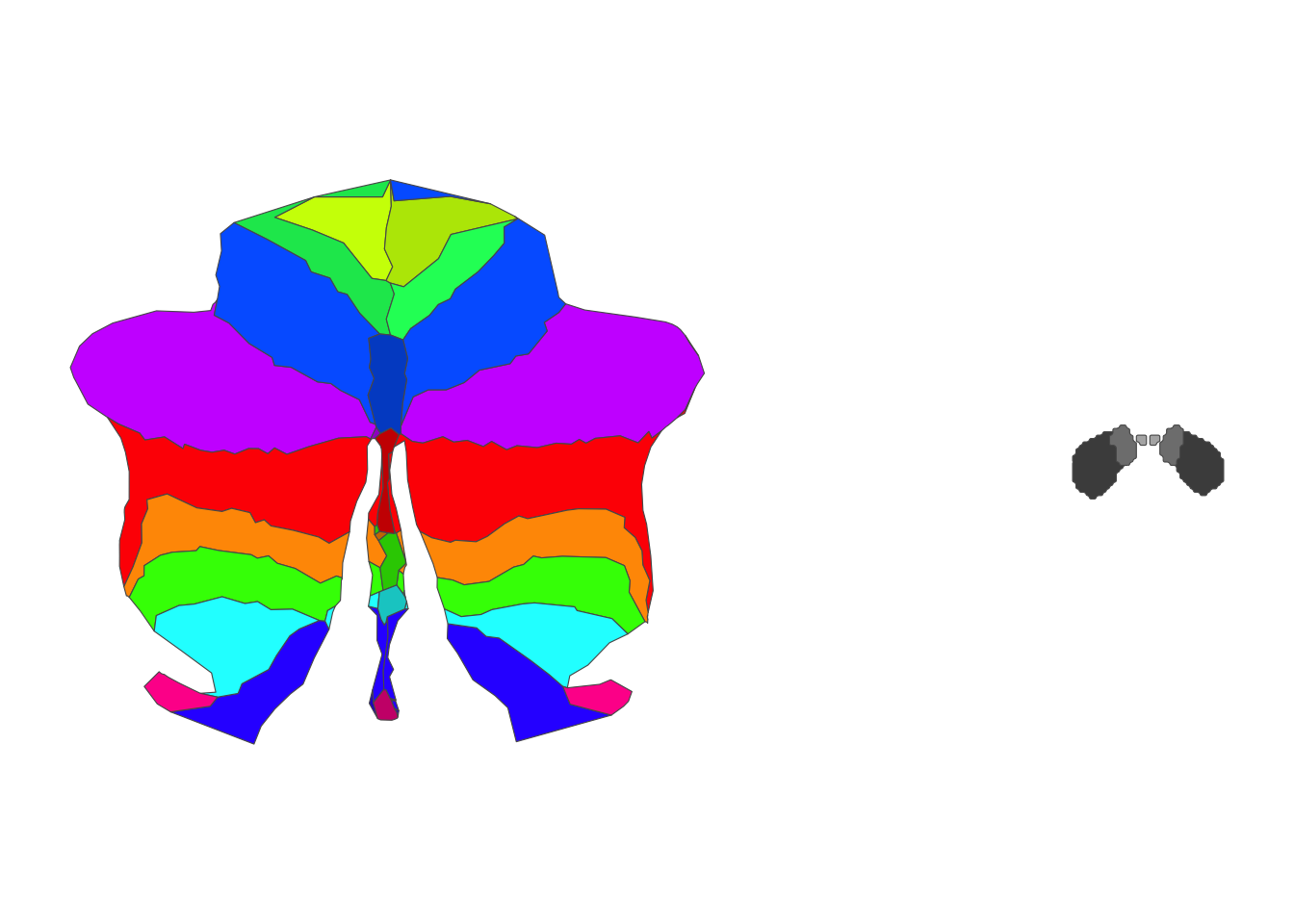
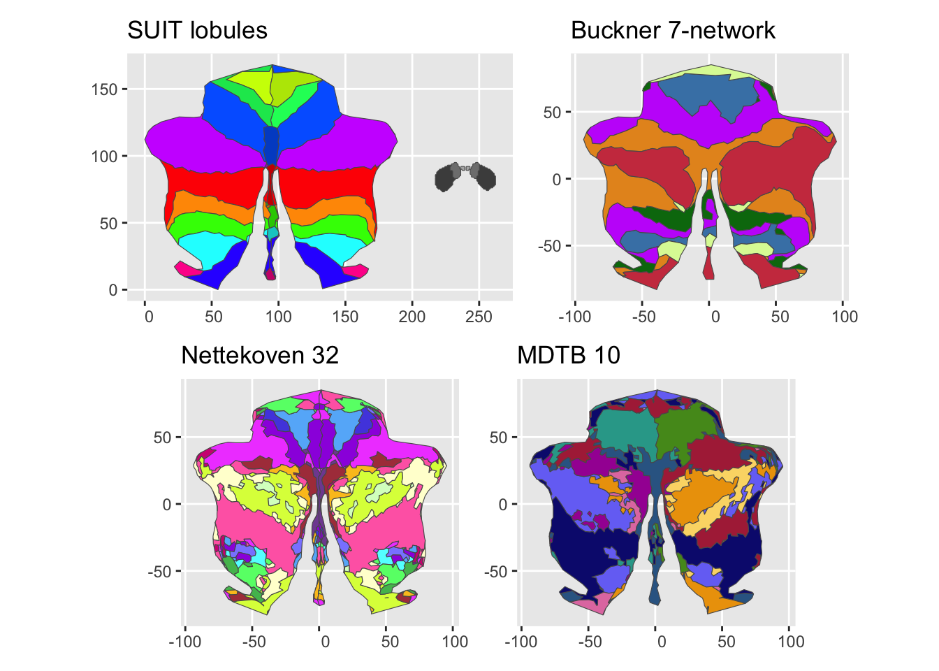
Cerebellar atlases work with geom_brain() exactly like cortical or subcortical ones. The atlas type determines the rendering — you don’t need to think about it.

library(ggseg)
library(ggsegSUIT)
library(ggsegCerebellum)
library(ggplot2)

ggplot() +
  geom_brain(
    atlas = suit(),
    mapping = aes(fill = label),
    show.legend = FALSE
  ) +
  scale_fill_manual(
    values = suit()$palette,
    na.value = "grey80"
  ) +
  theme_void()

The SUIT anatomical lobule atlas rendered as a flatmap.

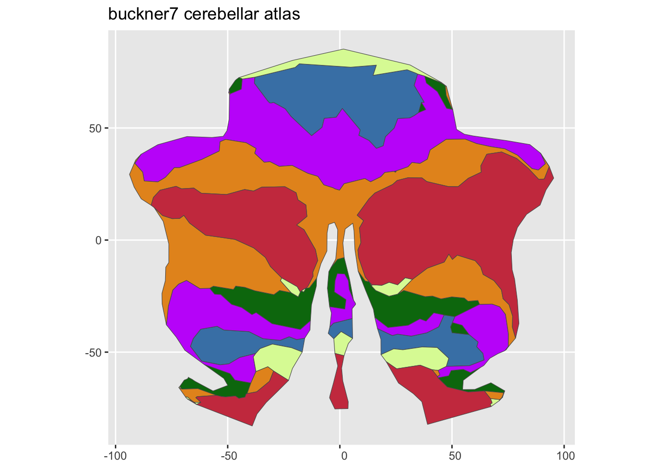
The plot() shorthand works too:

plot(buckner7())

Buckner 7-network cerebellar parcellation.

3D rendering with ggseg3d

The same atlas object renders in 3D without any conversion. Cerebellar atlases use vertex-based coloring on the SUIT surface — each region is a set of vertex indices painted onto a shared mesh.

library(ggseg3d)

ggseg3d(atlas = suit()) |>
  pan_camera("superior")

The SUIT anatomical lobule atlas in 3D. Rotate to explore.

Some cerebellar parcellations include deep nuclei — the Dentate, Interposed, and Fastigial nuclei buried inside the cerebellar white matter. These structures don’t live on the SUIT surface, so ggseg3d renders them as separate meshes, with the surface drawn at reduced opacity to let you see through to the nuclei underneath.

The SUIT atlas includes all six deep nuclei (Dentate, Interposed, and Fastigial, bilaterally). When these are present, the cortical surface becomes translucent so the nuclei are visible inside:

ggseg3d(atlas = suit()) |>
  set_background("#1a1a2e") |>
  pan_camera("left lateral")

Deep cerebellar nuclei rendered inside a translucent SUIT surface. The Dentate nucleus is the largest structure visible.

Multiple atlases out of the box

The anatomical lobule atlas lives in ggsegSUIT, while ggsegCerebellum ships seven functional and task-based parcellations from the Diedrichsen Lab’s cerebellar atlas collection:

library(patchwork)

p1 <- plot(suit()) + ggtitle("SUIT lobules")
p2 <- plot(buckner7()) + ggtitle("Buckner 7-network")
p3 <- plot(nettekoven32()) + ggtitle("Nettekoven 32")
p4 <- plot(mdtb10()) + ggtitle("MDTB 10")

(p1 + p2) / (p3 + p4)

Four cerebellar atlases: SUIT anatomical lobules plus three functional parcellations from ggsegCerebellum.

The full set across both packages:

• ggsegSUIT::suit() — SUIT anatomical lobules and deep nuclei (34 regions)
• buckner7() — Buckner 7-network functional parcellation
• buckner17() — Buckner 17-network functional parcellation
• ji10() — Ji 10-network subcortical parcellation
• mdtb10() — King MDTB 10-region task-based parcellation
• xue10() — Xue 10-network individual parcellation
• nettekoven32() — Nettekoven 32-region hierarchical parcellation
• nettekoven68() — Nettekoven 68-region hierarchical parcellation

Mapping your own data

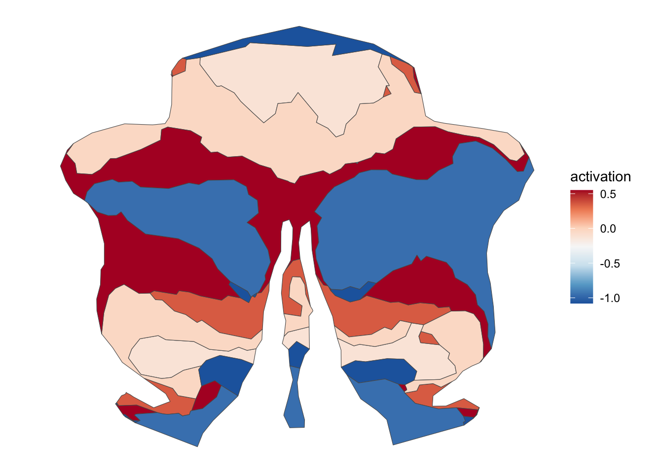
Plotting an atlas is step one. The real use case is mapping your own results onto the cerebellum — activation maps, connectivity values, anything region-based.

my_data <- data.frame(
  label = as.data.frame(buckner7())$label |> unique() |> na.omit(),
  activation = rnorm(7)
)

ggplot(my_data) +
  geom_brain(
    atlas = buckner7(),
    mapping = aes(fill = activation)
  ) +
  scale_fill_distiller(palette = "RdBu") +
  theme_void()

Merging atlas and data by label.

Simulated activation data mapped onto the Buckner 7-network cerebellar parcellation.

Building custom cerebellar atlases

If your parcellation isn’t one of the eight bundled atlases, ggseg.extra provides three pipelines for creating your own. The right one depends on what format your data lives in.

From GIFTI labels

Most cerebellar parcellations from the Diedrichsen Lab ship as GIFTI files mapped onto the SUIT surface. This is the simplest path — no FreeSurfer, no coordinate transforms.

library(ggseg.extra)

atlas <- create_cerebellar_from_gifti(
  gifti_files = "my_parcellation.label.gii",
  atlas_name = "my_cerebellum"
)

plot(atlas)

From MNI-space volumes

Many cerebellar parcellations exist as NIfTI volumes in MNI space. The pipeline handles the coordinate transform to SUIT space for you — download the deformation field once, then warp as many volumes as you need.

xfm <- suit_deformation_field(template = "MNI152NLin6AsymC")

suit_vol <- transform_mni_to_suit(
  input_volume = "my_parcellation.nii.gz",
  deformation_field = xfm,
  interpolation = "nearest"
)

atlas <- create_cerebellar_from_volume(
  volume = suit_vol,
  atlas_name = "my_mni_cerebellum"
)

From FreeSurfer annotations

If your parcellation lives as a FreeSurfer .annot file on the SUIT surface:

atlas <- create_cerebellar_from_annotation(
  annot = "my_parcellation.annot",
  atlas_name = "my_annot_cerebellum"
)

All three pipelines produce the same unified atlas object — 2D flatmap geometry, 3D vertex indices, and a color palette ready for both renderers.

Under the hood

A few implementation details that might matter if you’re building atlases or contributing to the ecosystem.

Boundary triangle splitting. Where two or three atlas regions meet on the SUIT surface, triangles span region boundaries. The pipeline splits these triangles at edge midpoints to eliminate sawtooth artifacts. The result is clean region boundaries in both 2D and 3D.

Deep nuclei as separate meshes. Structures like the Dentate nucleus don’t have vertices on the SUIT surface — they’re embedded in white matter. The pipeline tessellates them as individual 3D meshes (like subcortical structures) and renders them alongside the surface.

Orphaned region rescue. Some parcellations have tiny regions that don’t map to any SUIT vertex. Rather than dropping them silently, the pipeline assigns them to their nearest surface neighbor so they remain visible.

What’s where

The cerebellar work touches four packages:

Package	What changed	CRAN
ggseg.formats	New cerebellar atlas type and data container	Yes
ggseg	2D stacking support for flatmap view	Yes
ggseg3d	3D rendering with vertex coloring and deep nuclei	Yes
ggseg.extra	Three creation pipelines, SUIT surfaces, MNI-to-SUIT transforms	Pending

ggseg.formats, ggseg, and ggseg3d are already on CRAN. ggseg.extra will follow once an upstream dependency (freesurfer) merges our PRs — the volume pipeline needs functions from our fork.

In the meantime, install everything from r-universe:

install.packages(
  c("ggseg.formats", "ggseg", "ggseg3d", "ggseg.extra", "ggsegSUIT", "ggsegCerebellum"),
  repos = c(
    "https://ggseg.r-universe.dev",
    "https://cloud.r-project.org"
  )
)

The bigger picture

The cerebellum is having a moment in neuroimaging. Functional connectivity studies keep finding cerebellar contributions to cognition, language, and emotion — far beyond the traditional motor-only story. Tools like SUIT and the cerebellar atlas collection have made cerebellar analysis accessible.

ggseg can now keep up. If you’re working with cerebellar data, your visualizations no longer need a separate toolchain. Same geom_brain(), same ggseg3d(), same atlas object — just a different brain region.

We’d love to hear how you use it. Open a discussion or file an issue if something doesn’t work the way you expect.