library(ggseg)
library(ggplot2)
ggplot() +
geom_brain(
atlas = dk(),
aes(fill = region),
show.legend = FALSE
) +
theme_void()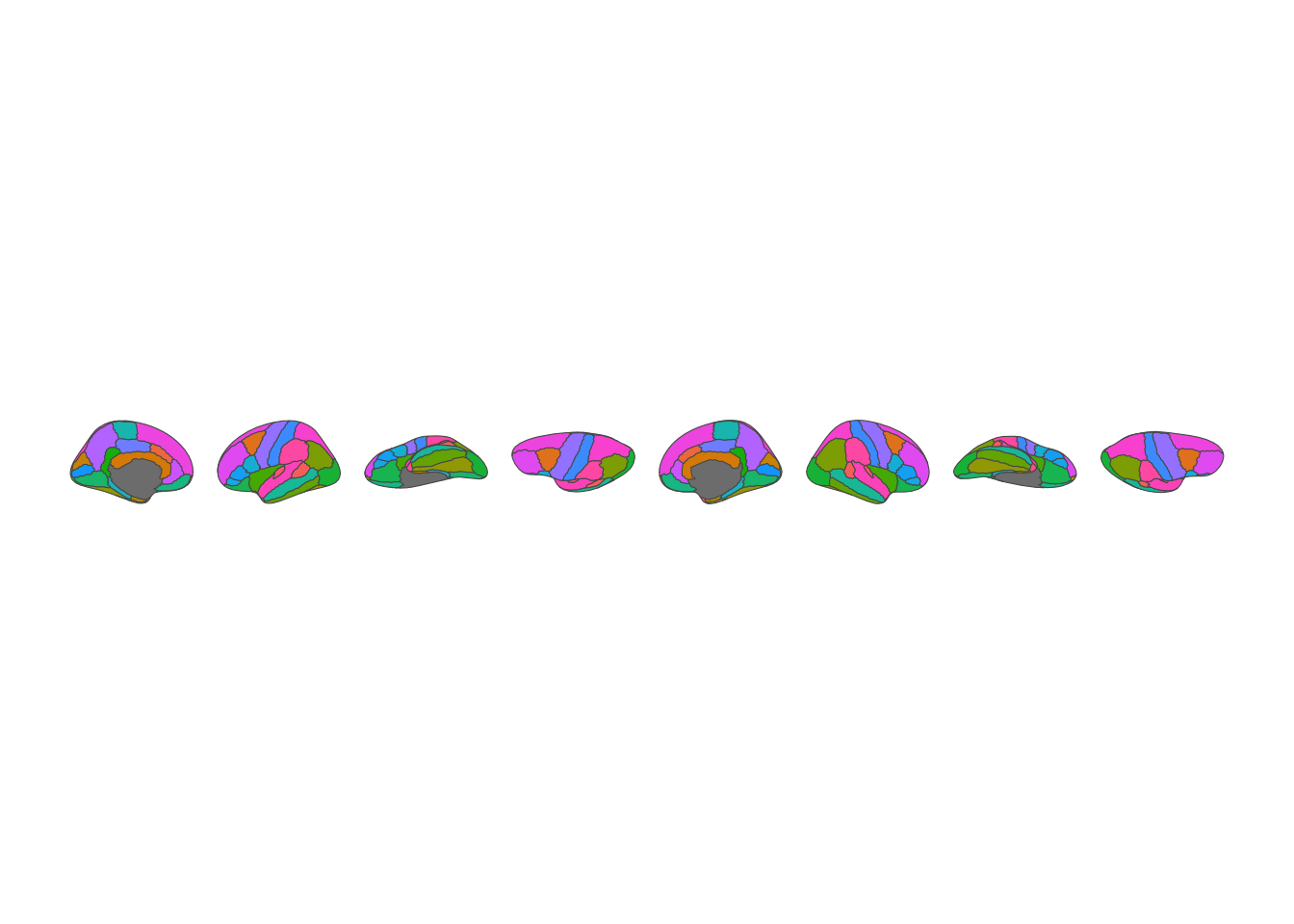
If you’ve used ggseg for any length of time, you know the ceremony. You load ggseg for your 2D figures. You load ggseg3d for the 3D ones. You remember that the 2D atlas is called dk, but the 3D version is dk_3d. You keep both objects in your head, hoping they agree on region names. They usually do. Usually.
That entire dance is over. ggseg 2.0 ships a single, unified atlas format that works for both 2D and 3D visualization. One object. Both renderers. No suffix juggling.
The old atlas format stored full 3D mesh geometry per region. Every cortical region carried its own copy of vertex coordinates and face indices — duplicating data that was mostly shared across the brain surface. Subcortical structures stored dense meshes straight from the segmentation. White matter tracts had no 3D representation at all.
The new format rethinks storage for each atlas type:
Cortical atlases store integer vertex indices instead of mesh geometry. Each region is just a vector of integers pointing into a shared fsaverage5 template mesh (10,242 vertices per hemisphere). The mesh itself lives once in ggseg.formats, not in every atlas package. The size difference is dramatic — a list of integers vs. thousands of duplicated 3D coordinates.
Subcortical atlases use decimated meshes. The raw marching-cubes output from volumetric segmentation is simplified to a fraction of the original face count while preserving shape. Smaller objects, faster rendering, same visual quality.
Tract atlases now have 3D support for the first time. Centerline geometry extracted from tractography streamlines is stored as tube centerlines rather than raw meshes. This is entirely new — tracts in ggseg v1 were 2D only.
The practical result: atlas packages shrink, install faster, and render faster. Plotting a cortical atlas in 3D loads one shared mesh and colors vertices by index lookup instead of assembling dozens of separate meshes. That’s a win at every level — package size on disk, download time, memory at runtime, and time to first plot.
Four packages were rewritten or substantially reworked. Here’s what happened and why it matters.
The biggest structural change is a new package called ggseg.formats that defines a single ggseg_atlas S3 class. Every atlas — cortical, subcortical, or white matter tract — now lives in one object that carries everything both renderers need: sf geometries for 2D plotting, vertex indices or meshes for 3D, region metadata, and a color palette.
library(ggseg)
library(ggplot2)
ggplot() +
geom_brain(
atlas = dk(),
aes(fill = region),
show.legend = FALSE
) +
theme_void()
library(ggseg3d)
ggseg3d(atlas = dk()) |>
pan_camera("right lateral")The same dk atlas rendered in 3D
The separate _3d objects are gone. If your code references dk_3d or aseg_3d, it will need updating — but the change is mechanical and the error messages will tell you what to do.
The 3D renderer was rebuilt from scratch. plotly served well for years, but it struggled with the size of brain meshes and gave limited control over rendering. Plotly has also been retiring its R documentation and support, focusing resources on Python — not a foundation we want to build on going forward. The new engine uses Three.js through htmlwidgets, which means better performance, lower memory use, and a proper API for controlling the scene.
New capabilities include orthographic projection, glassbrain overlays, flat shading for exact color matching, edge rendering for region boundaries, and standard anatomical camera positions. The API is pipe-friendly:
ggseg3d(atlas = aseg()) |>
set_background("#1a1a2e") |>
set_flat_shading() |>
add_glassbrain() |>
pan_camera("left lateral")