from plotnine import ggplot
from ggsegpy import geom_brain, dk

ggplot() + geom_brain(atlas=dk())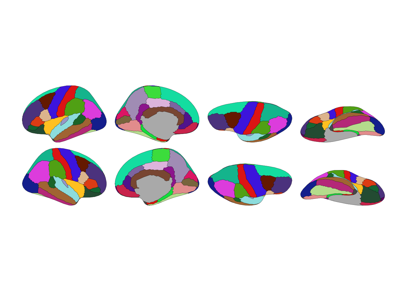
The 2D plots use plotnine, Python’s implementation of ggplot2. If you know ggplot2 from R, you’re already home. If you don’t, the grammar-of-graphics approach means plots build up from layers—data, aesthetics, geometries, scales, themes.
from plotnine import ggplot
from ggsegpy import geom_brain, dk
ggplot() + geom_brain(atlas=dk())
Often you only need one hemisphere:
ggplot() + geom_brain(atlas=dk(), hemi="left")
ggplot() + geom_brain(atlas=dk(), hemi="right")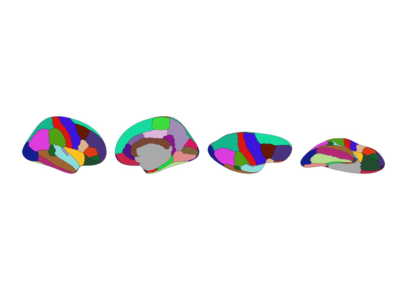
Each hemisphere has lateral (outside) and medial (inside) views:
ggplot() + geom_brain(atlas=dk(), hemi="left", view="lateral")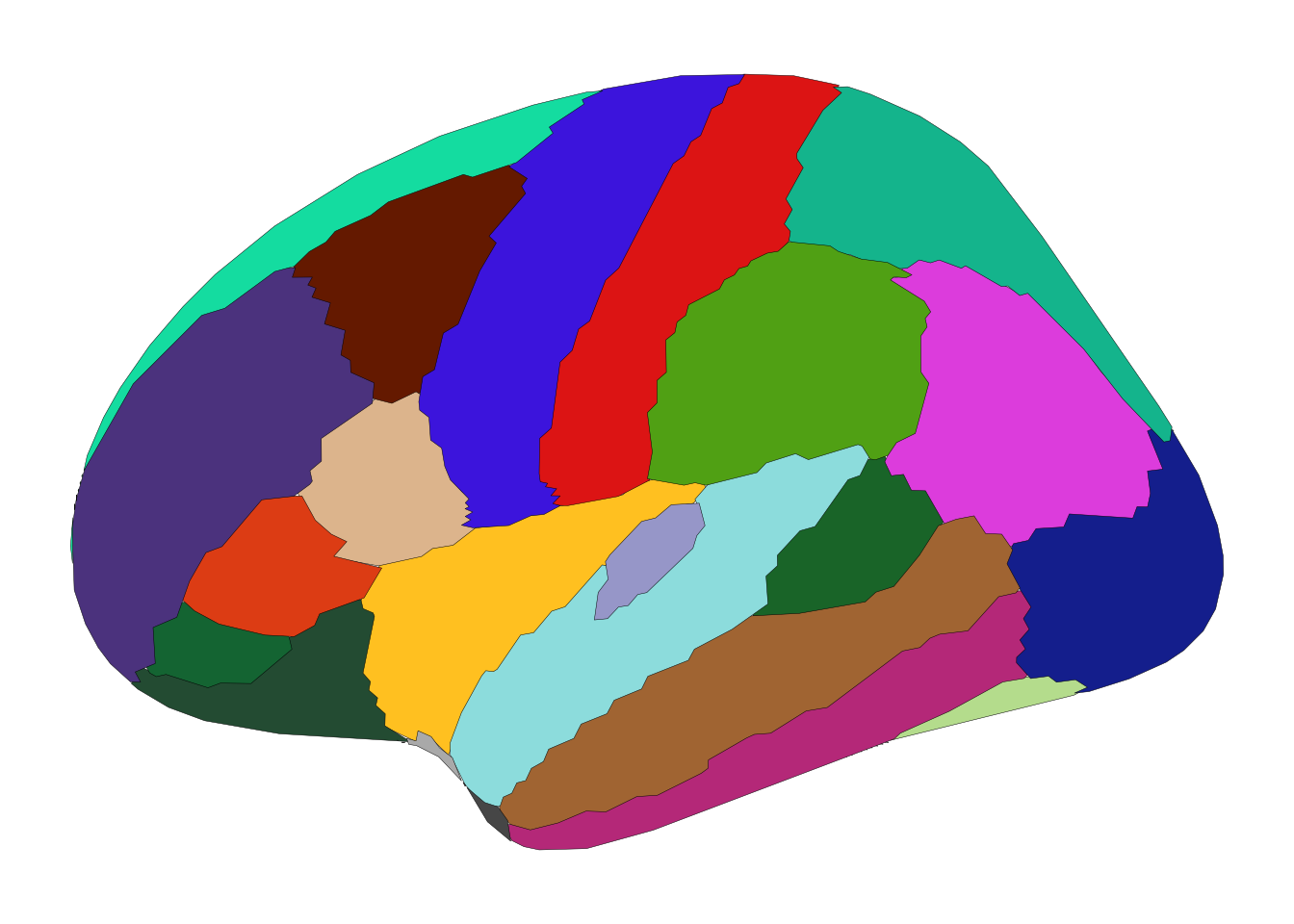
ggplot() + geom_brain(atlas=dk(), hemi="left", view="medial")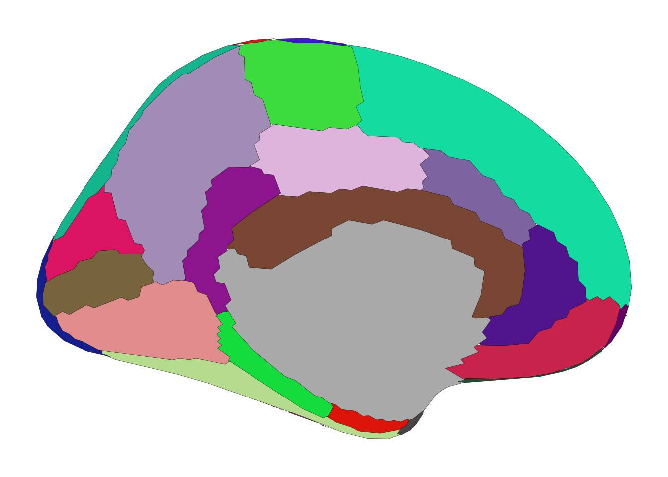
ggsegpy ships with themes designed for brain plots:
from ggsegpy import theme_brain, theme_brain_void, theme_darkbrain

p = ggplot() + geom_brain(atlas=dk(), hemi="left")
p + theme_brain()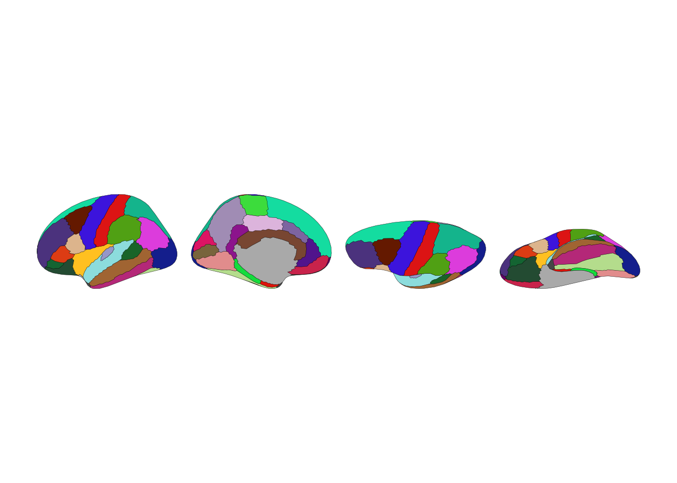
p + theme_brain_void()
p + theme_darkbrain()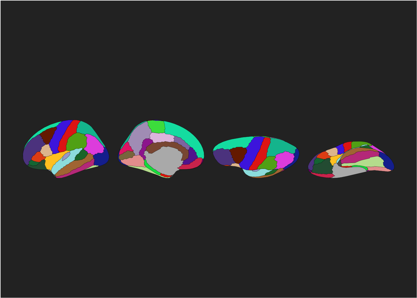
Since geom_brain() works with plotnine, you can add any plotnine layer:
from plotnine import labs, theme, element_text

p = ggplot() + geom_brain(atlas=dk(), hemi="left")
p + labs(title="Desikan-Killiany Atlas", subtitle="Left hemisphere")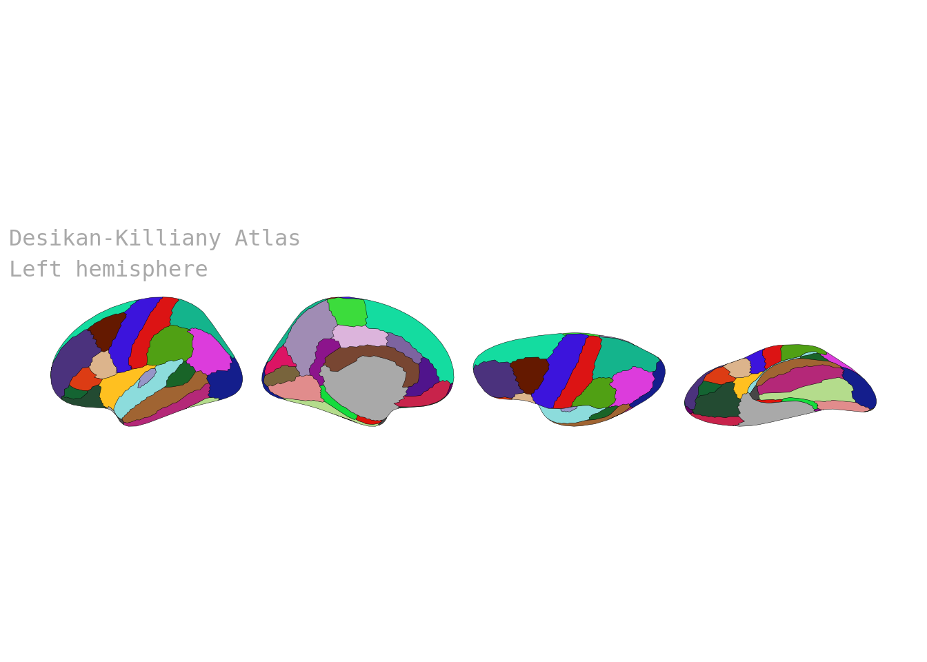
The aseg atlas shows subcortical structures in axial slices. The grey outline is the cortex, providing spatial context:
from ggsegpy import aseg

ggplot() + geom_brain(atlas=aseg())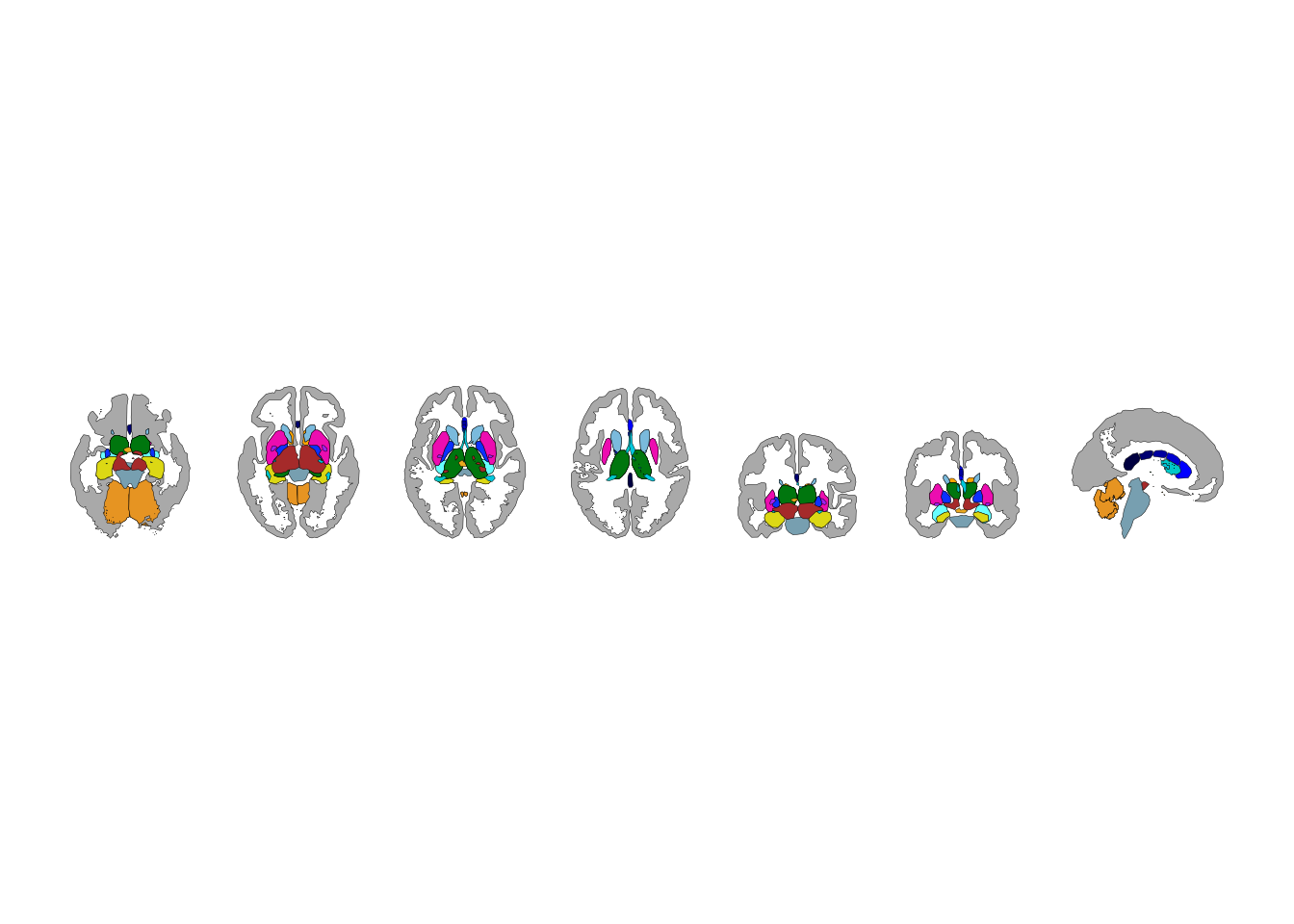
White matter tracts from TRACULA:
from ggsegpy import tracula

ggplot() + geom_brain(atlas=tracula())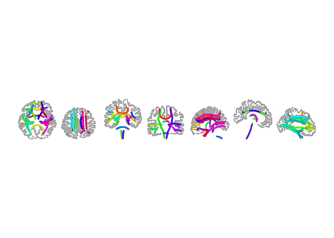
p = ggplot() + geom_brain(atlas=dk())
p.save("dk_atlas.png", width=10, height=4, dpi=300)
For publication figures, 300 DPI and explicit dimensions give you control over the final output.