The whole point of brain visualization is showing your own data—cortical thickness, activation maps, effect sizes.
The join
Your data needs a column that matches labels in the atlas:
import pandas as pd
from ggsegpy import dk, brain_join

atlas = dk()

my_data = pd.DataFrame({
    "label": ["lh_precentral", "lh_postcentral", "rh_precentral", "rh_postcentral"],
    "thickness": [2.5, 2.1, 2.4, 2.0]
})

merged = brain_join(my_data, atlas)
merged[["label", "hemi", "region", "thickness"]].head()
| 0 |
lh_bankssts |
left |
banks of superior temporal sulcus |
NaN |
| 1 |
lh_caudalmiddlefrontal |
left |
caudal middle frontal |
NaN |
| 2 |
lh_corpuscallosum |
left |
corpus callosum |
NaN |
| 3 |
lh_entorhinal |
left |
entorhinal |
NaN |
| 4 |
lh_frontalpole |
left |
frontal pole |
NaN |
The join is a left join—every atlas region appears, with NaN for regions not in your data.
Joining by label
Labels follow the pattern {hemisphere}_{region}:
from plotnine import ggplot, aes
from ggsegpy import geom_brain
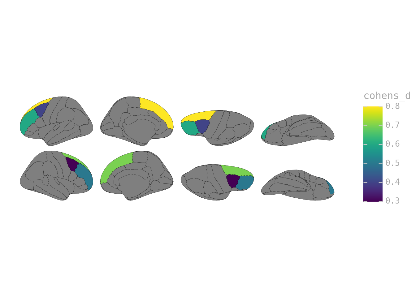
effect_sizes = pd.DataFrame({
"label": [
"lh_superiorfrontal", "lh_rostralmiddlefrontal", "lh_caudalmiddlefrontal",
"rh_superiorfrontal", "rh_rostralmiddlefrontal", "rh_caudalmiddlefrontal"
],
"cohens_d": [0.8, 0.6, 0.4, 0.7, 0.5, 0.3]
})
ggplot(effect_sizes) + geom_brain(atlas=dk(), mapping=aes(fill="cohens_d"))
Joining by region
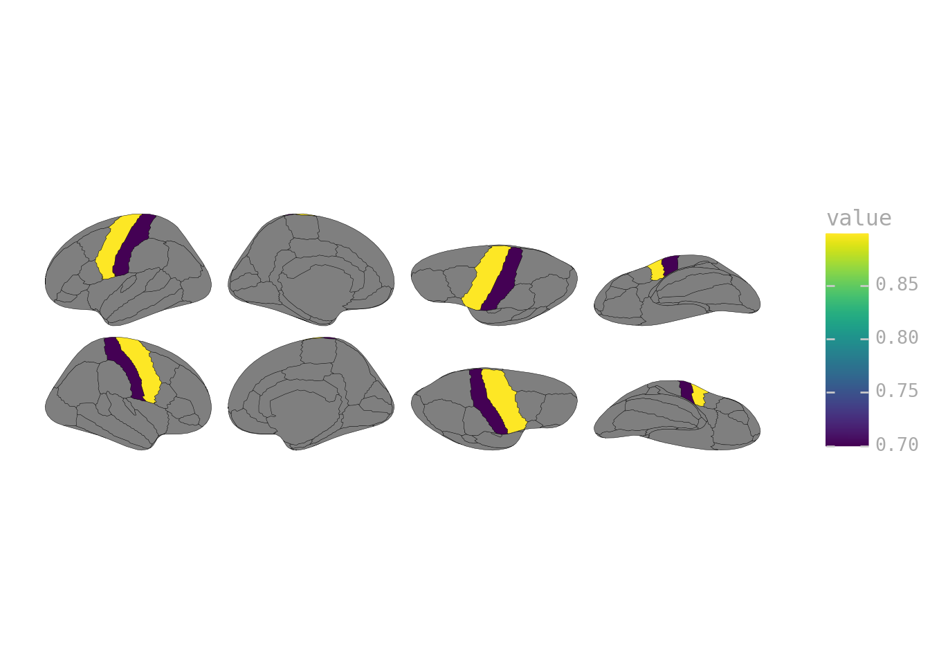
If your data doesn’t distinguish hemispheres, join by region name:
region_data = pd.DataFrame({
    "region": ["precentral", "postcentral", "superiorfrontal"],
    "value": [0.9, 0.7, 0.5]
})

ggplot(region_data) + geom_brain(atlas=dk(), mapping=aes(fill="value"))
Both hemispheres get the same color—what you want when your analysis collapsed across hemispheres.
Color scales
Since geom_brain returns a plotnine object, add any ggplot2-style scale:
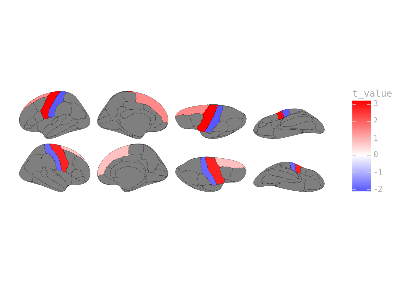
from plotnine import scale_fill_gradient2

activation_data = pd.DataFrame({
    "label": ["lh_precentral", "lh_postcentral", "lh_superiorfrontal",
              "rh_precentral", "rh_postcentral", "rh_superiorfrontal"],
    "t_value": [3.2, -2.1, 1.5, 2.8, -1.9, 0.8]
})

p = ggplot(activation_data) + geom_brain(atlas=dk(), mapping=aes(fill="t_value"))
p + scale_fill_gradient2(low="blue", mid="white", high="red", midpoint=0)
from plotnine import scale_fill_cmap

p = ggplot(effect_sizes) + geom_brain(atlas=dk(), mapping=aes(fill="cohens_d"))
p + scale_fill_cmap(cmap_name="viridis")
3D with custom data
Same pattern—use color parameter:
from ggsegpy import ggseg3d, pan_camera

fig = ggseg3d(data=effect_sizes, atlas=dk(), color="cohens_d")
fig = pan_camera(fig, "left lateral")
fig
Subcortical data
Check available labels:
from ggsegpy import aseg

aseg_atlas = aseg()
print(aseg_atlas.labels[:10])
['Left-Cerebellum-Cortex', 'Right-Cerebellum-Cortex', 'cortex_', 'Brain-Stem', 'CC_Mid_Posterior', 'Left-Accumbens-area', 'Left-Amygdala', 'Left-Caudate', 'Left-Hippocampus', 'Left-Pallidum']
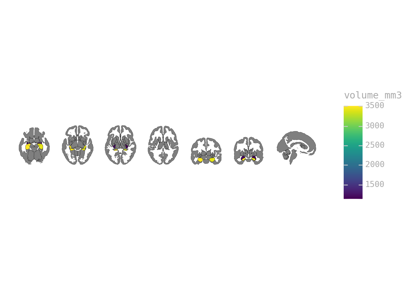
volumes = pd.DataFrame({
    "label": ["Left-Hippocampus", "Right-Hippocampus", "Left-Amygdala", "Right-Amygdala"],
    "volume_mm3": [3500, 3400, 1200, 1150]
})

ggplot(volumes) + geom_brain(atlas=aseg(), mapping=aes(fill="volume_mm3"))
Troubleshooting
If your plot looks wrong, check the join:
bad_data = pd.DataFrame({
    "label": ["precentral", "postcentral"],  # Missing hemisphere prefix
    "value": [1.0, 2.0]
})

merged = brain_join(bad_data, dk())
The warning tells you which labels didn’t match.
Quick reference
Every atlas has a .labels property:
from ggsegpy import dk, aseg, tracula

print("DK labels (first 5):", dk().labels[:5])
print("ASEG labels (first 5):", aseg().labels[:5])
print("TRACULA labels (first 5):", tracula().labels[:5])
DK labels (first 5): ['lh_bankssts', 'lh_caudalmiddlefrontal', 'lh_corpuscallosum', 'lh_entorhinal', 'lh_frontalpole']
ASEG labels (first 5): ['Left-Cerebellum-Cortex', 'Right-Cerebellum-Cortex', 'cortex_', 'Brain-Stem', 'CC_Mid_Posterior']
TRACULA labels (first 5): ['cortex_', 'acomm.bbr.prep', 'cc.bodyt.bbr.prep', 'cc.genu.bbr.prep', 'cc.rostrum.bbr.prep']