from plotnine import ggplot
from ggsegpy import geom_brain, dk

ggplot() + geom_brain(atlas=dk())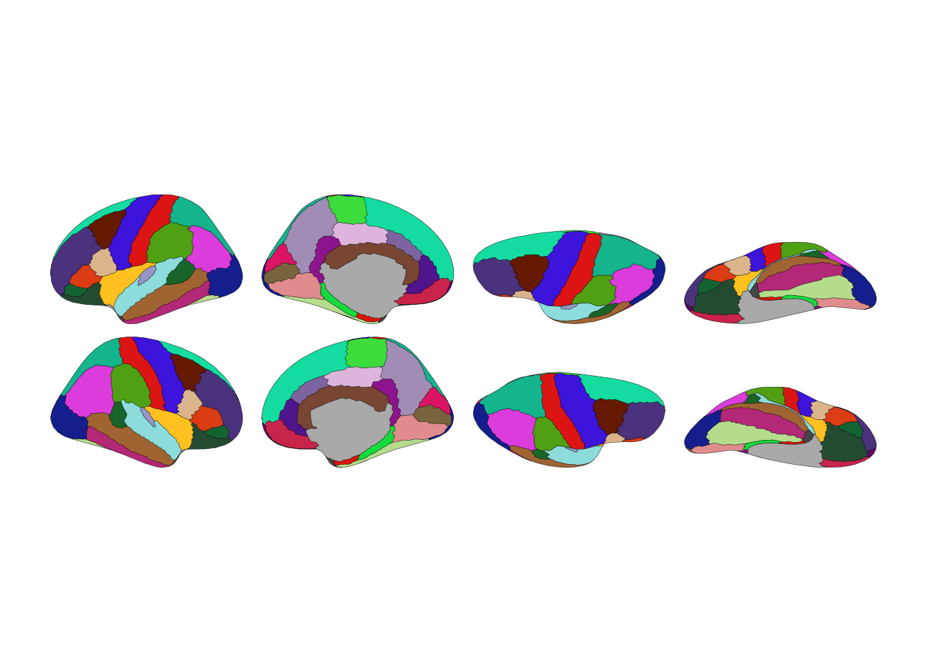
pip install ggsegpyOr install from source:
pip install git+https://github.com/ggsegverse/ggsegpy.gitggsegpy requires:
These install automatically with pip.
from plotnine import ggplot
from ggsegpy import geom_brain, dk
ggplot() + geom_brain(atlas=dk())
That’s the Desikan-Killiany atlas—34 cortical regions per hemisphere. Each color is a brain region. Grey areas are the medial wall, shown for context.
Three atlases ship with ggsegpy:
from ggsegpy import dk, aseg, tracula

# Cortical parcellation
print(f"dk: {len(dk().labels)} labels")

# Subcortical segmentation
print(f"aseg: {len(aseg().labels)} labels")

# White matter tracts
print(f"tracula: {len(tracula().labels)} labels")
dk: 72 labels
aseg: 30 labels
tracula: 45 labelsggplot() + geom_brain(atlas=dk())
ggplot() + geom_brain(atlas=aseg())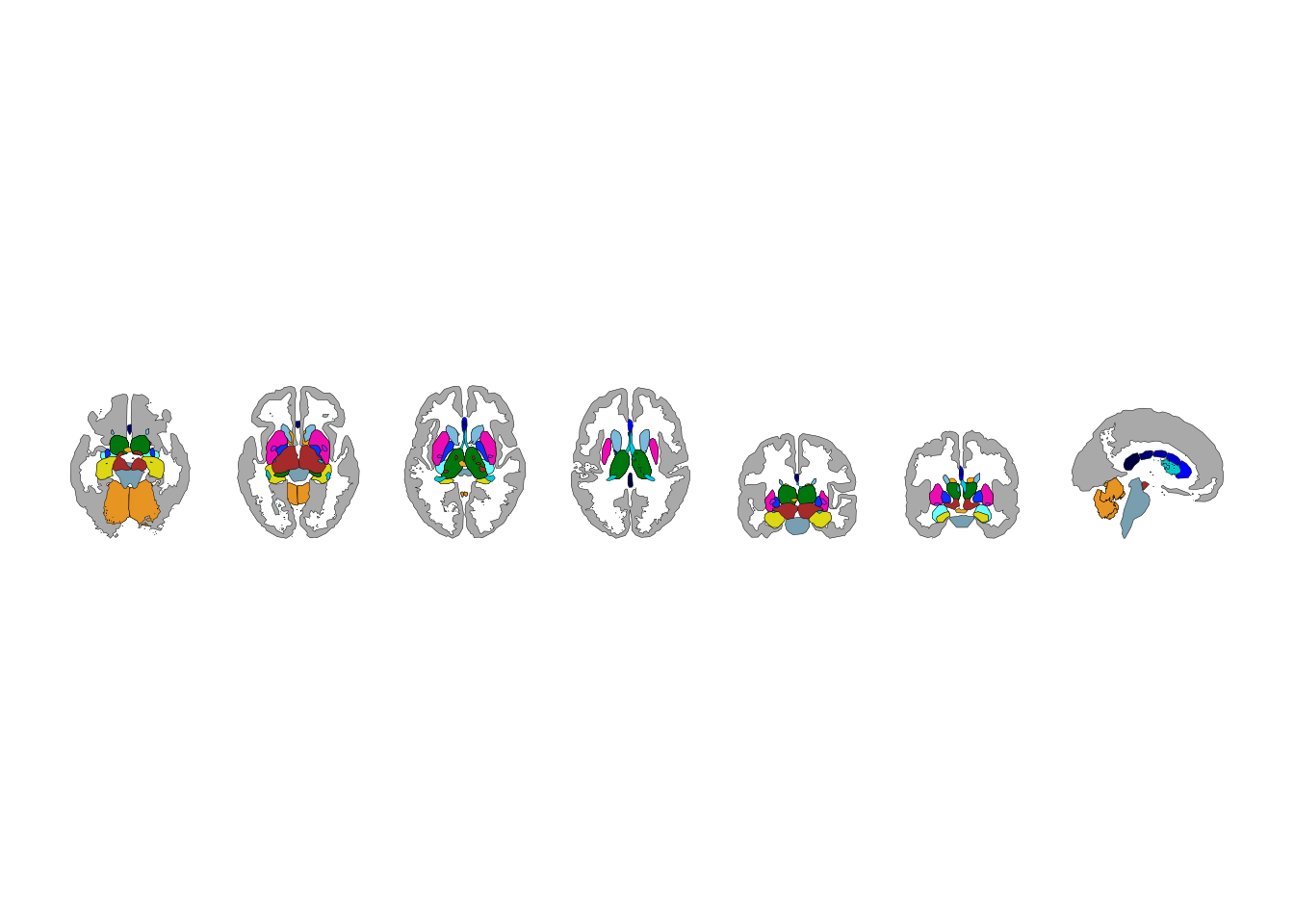
ggplot() + geom_brain(atlas=tracula())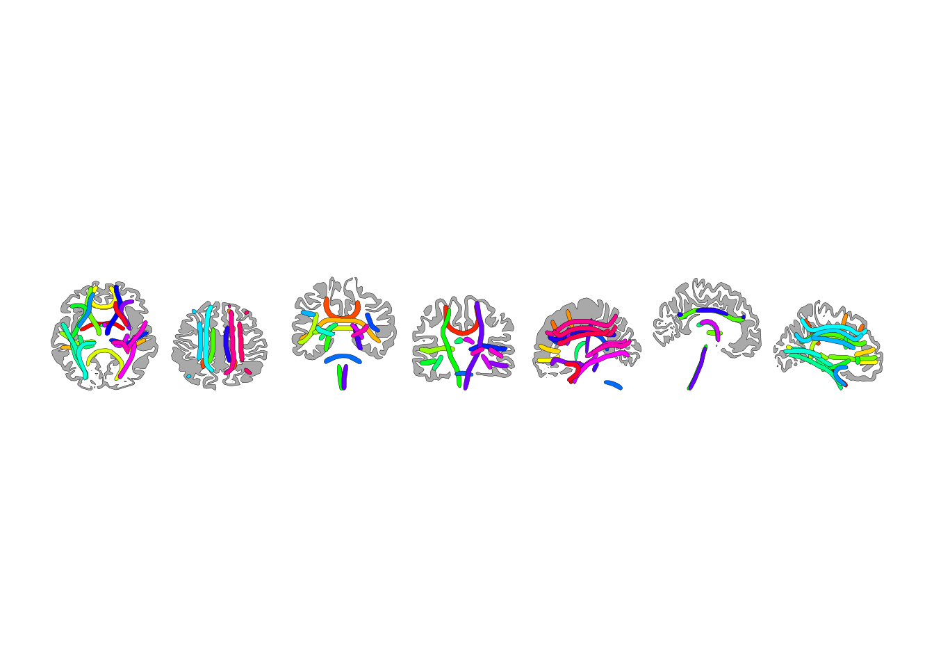
Every atlas works in both 2D and 3D. Use ggseg3d() for interactive 3D:
from ggsegpy import ggseg3d

ggseg3d(atlas=dk())The real point is visualizing your own data. Pass a DataFrame with labels matching the atlas:
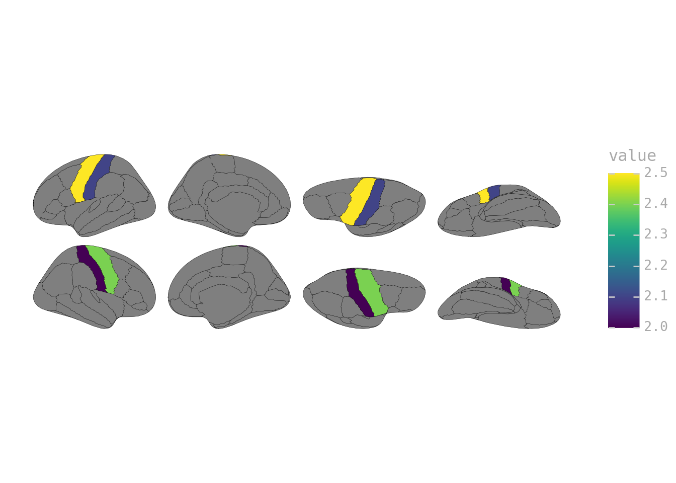
from plotnine import ggplot, aes
import pandas as pd

my_data = pd.DataFrame({
    "label": ["lh_precentral", "lh_postcentral", "rh_precentral", "rh_postcentral"],
    "value": [2.5, 2.1, 2.4, 2.0]
})

ggplot(my_data) + geom_brain(atlas=dk(), mapping=aes(fill="value"))