Subcortical atlases represent the structures beneath the cortical surface: thalamus, hippocampus, amygdala, caudate, putamen, and others. They come from volumetric segmentations like FreeSurfer’s aseg.mgz, where each voxel is assigned a label.
The pipeline tessellates labelled voxel regions into 3D meshes and (optionally) creates 2D projection views that collapse a slab of the volume onto a single plane.
This tutorial recreates the aseg atlas — the same pipeline behind data-raw/make_aseg_atlas.R in ggseg.formats.
What you need
- FreeSurfer installed with the
fsaverage5subject - ImageMagick for 2D geometry extraction
- Chrome/Chromium for 3D screenshots
Creating the atlas
create_subcortical_from_volume() takes a segmentation volume and a colour lookup table. The pipeline tessellates each labelled region into a 3D mesh, then creates 2D projection views:
aseg_raw <- create_subcortical_from_volume(
  input_volume = aseg_volume,
  input_lut = color_lut,
  atlas_name = "aseg"
)
#> Warning: Atlas has 11943 vertices (threshold:
#> 10000)
#> ℹ Large atlases may be slow to plot and
#>   increase package size
#> ℹ Call `atlas_smooth(atlas, keep = 0.2,
#>   exclude = "cortex_")` to reduce vertices

aseg_raw
#>
#> ── aseg ggseg atlas ──────────────────────
#> Type: subcortical
#> Regions: 27
#> Hemispheres: left, NA, right
#> Views: axial_1, axial_2, axial_3,
#> axial_4, axial_5, axial_6, axial_7,
#> coronal_1, coronal_2, coronal_3,
#> coronal_4, coronal_5, sagittal
#> Palette: ✔
#> Rendering: ✔ ggseg
#> ✔ ggseg3d (meshes)
#> ──────────────────────────────────────────
#> # A tibble: 43 × 3
#>    hemi  region                  label
#>    <chr> <chr>                   <chr>
#>  1 left  cerebral white matter   Left-Cer…
#>  2 left  cerebral cortex         Left-Cer…
#>  3 left  lateral ventricle       Left-Lat…
#>  4 left  inf lat vent            Left-Inf…
#>  5 left  cerebellum white matter Left-Cer…
#>  6 left  cerebellum cortex       Left-Cer…
#>  7 left  thalamus                Left-Tha…
#>  8 left  caudate                 Left-Cau…
#>  9 left  putamen                 Left-Put…
#> 10 left  pallidum                Left-Pal…
#> 11 <NA>  3rd ventricle           3rd-Vent…
#> 12 <NA>  4th ventricle           4th-Vent…
#> 13 <NA>  brain stem              Brain-St…
#> 14 left  hippocampus             Left-Hip…
#> 15 left  amygdala                Left-Amy…
#> 16 <NA>  csf                     CSF
#> 17 left  accumbens area          Left-Acc…
#> 18 left  ventraldc               Left-Ven…
#> 19 left  vessel                  Left-ves…
#> 20 left  choroid plexus          Left-cho…
#> 21 right cerebral white matter   Right-Ce…
#> 22 right cerebral cortex         Right-Ce…
#> 23 right lateral ventricle       Right-La…
#> 24 right inf lat vent            Right-In…
#> 25 right cerebellum white matter Right-Ce…
#> 26 right cerebellum cortex       Right-Ce…
#> 27 right thalamus                Right-Th…
#> 28 right caudate                 Right-Ca…
#> 29 right putamen                 Right-Pu…
#> 30 right pallidum                Right-Pa…
#> 31 right hippocampus             Right-Hi…
#> 32 right amygdala                Right-Am…
#> 33 right accumbens area          Right-Ac…
#> 34 right ventraldc               Right-Ve…
#> 35 right vessel                  Right-ve…
#> 36 right choroid plexus          Right-ch…
#> 37 <NA>  wm hypointensities      WM-hypoi…
#> 38 <NA>  optic chiasm            Optic-Ch…
#> 39 <NA>  cc posterior            CC_Poste…
#> 40 <NA>  cc mid posterior        CC_Mid_P…
#> 41 <NA>  cc central              CC_Centr…
#> 42 <NA>  cc mid anterior         CC_Mid_A…
#> 43 <NA>  cc anterior             CC_Anter…
The default pipeline creates six projection views focused on the subcortical range: axial inferior, axial superior, coronal posterior, coronal anterior, sagittal left, and sagittal right. Each view collapses a slab of the volume onto a single plane, giving you spatial context without the complexity of individual slices.
Removing unwanted regions
The aseg segmentation contains everything — cortex, white matter, ventricles, CSF. For a subcortical atlas, most of these are noise. Remove them:
aseg_raw <- aseg_raw |>
  atlas_region_remove("White-Matter", match_on = "label") |>
  atlas_region_remove("WM-hypointensities", match_on = "label") |>
  atlas_region_remove("-Ventricle", match_on = "label") |>
  atlas_region_remove("-Vent$", match_on = "label") |>
  atlas_region_remove("CSF", match_on = "label") |>
  atlas_region_remove("Cerebral-Cortex", match_on = "label")
Patterns are regular expressions, so -Vent$ matches “3rd-Vent” and “4th-Vent” without catching “Ventral-DC.”
Setting context regions
The cortex works well as a background outline — it shows where subcortical structures sit relative to the brain surface without competing for colour:
aseg_raw <- aseg_raw |>
  atlas_region_contextual("Cortex", match_on = "label")
Selecting views
Not all projection views are equally useful. Keep the ones that show your structures best:
aseg_raw <- aseg_raw |>
  atlas_view_keep("axial_3|axial_5|coronal_2|coronal_3|coronal_4|sagittal")
Cleaning up the layout
Gather views into a compact arrangement:
aseg_raw <- aseg_raw |>
  atlas_view_gather()
The shortcut: aseg_context()
The remove → contextualise → view-keep → gather recipe above is the same for every subcortical atlas, so aseg_context() collapses it into one call. It punches the cortical white matter out of the brain silhouette, strips the structures aseg does not draw (aseg_hidden_labels()), demotes everything outside focus to grey context, and drops views with no focus region:
aseg_raw <- create_subcortical_from_volume(
  input_volume = aseg_volume,
  input_lut = color_lut,
  atlas_name = "aseg"
) |>
  aseg_context(
    focus = "Thalamus|Caudate|Putamen|Pallidum|Hippocampus|Amygdala|Accumbens|VentralDC|Brain-Stem"
  )
focus is matched with a loose, case-insensitive grepl(), so you don’t have to spell out FreeSurfer’s exact Left-/Right- label casing. The labels that don’t match become context, and demoting them uses a separate, exact, case-sensitive ^(...)$ match against their own resolved label strings — not focus re-applied — so a context label that happens to contain a focus label as a substring (the classic Thalamus inside hypothalamus) can never swallow it. That substring collision used to demote the whole focus set to context, silently producing 0-region atlases, before this exact-match step was added.
subcortical_slabs() derives the projection slabs from the bounding box of a set of labels, reading the volume in the same frame the builder uses, so the slabs always land on the right slices. You can pass its arguments as a list to slabs, and run aseg_context() in the same call via context:
aseg <- create_subcortical_from_volume(
  input_volume = aseg_volume,
  input_lut = color_lut,
  atlas_name = "aseg",
  slabs = list(labels = c(10:13, 17:18, 26, 49:54, 58), coronal = 3, axial = 2),
  context = list(focus = "Thalamus|Caudate|Putamen|Pallidum|Hippocampus|Amygdala")
)
create_wholebrain_from_volume() forwards both slabs and context through its subcortical_opts, so a whole-brain build gets the same treatment for free.
Adding metadata
The raw labels are technical identifiers like “Left-Thalamus-Proper.” Join human-readable names and structural groupings:
normalize_region <- function(x) {
  ifelse(
    is.na(x),
    NA_character_,
    x |>
      tolower() |>
      gsub("-", " ", x = _) |>
      gsub("_", " ", x = _) |>
      gsub("left |right ", "", x = _) |>
      trimws()
  )
}

aseg_metadata <- data.frame(
  region = c(
    "Thalamus-Proper", "Caudate", "Putamen", "Pallidum",
    "Hippocampus", "Amygdala", "Accumbens-area", "VentralDC",
    "Brain-Stem"
  ),
  label_pretty = c(
    "thalamus", "caudate", "putamen", "pallidum",
    "hippocampus", "amygdala", "nucleus accumbens", "ventral DC",
    "brain stem"
  ),
  structure = c(
    "diencephalon", "basal ganglia", "basal ganglia", "basal ganglia",
    "limbic", "limbic", "basal ganglia", "diencephalon",
    "brainstem"
  )
)

core_with_meta <- aseg_raw$core |>
  mutate(region_key = normalize_region(region)) |>
  left_join(
    aseg_metadata |>
      mutate(region_key = normalize_region(region)) |>
      select(region_key, label_pretty, structure),
    by = "region_key"
  ) |>
  mutate(region = coalesce(label_pretty, region)) |>
  select(hemi, region, label, structure)
Rebuilding and saving
Construct the final atlas from modified components:
aseg <- ggseg_atlas(
  atlas = aseg_raw$atlas,
  type = aseg_raw$type,
  palette = aseg_raw$palette,
  core = core_with_meta,
  data = aseg_raw$data
)

aseg
#>
#> ── aseg ggseg atlas ──────────────────────
#> Type: subcortical
#> Regions: 17
#> Hemispheres: left, NA, right
#> Views: axial_3, axial_5, coronal_2,
#> coronal_3, coronal_4, sagittal
#> Palette: ✔
#> Rendering: ✔ ggseg
#> ✔ ggseg3d (meshes)
#> ──────────────────────────────────────────
#> # A tibble: 27 × 4
#>    hemi  region            label structure
#>    <chr> <chr>             <chr> <chr>
#>  1 left  thalamus          Left… <NA>
#>  2 left  caudate           Left… basal ga…
#>  3 left  putamen           Left… basal ga…
#>  4 left  pallidum          Left… basal ga…
#>  5 <NA>  brain stem        Brai… brainstem
#>  6 left  hippocampus       Left… limbic
#>  7 left  amygdala          Left… limbic
#>  8 left  nucleus accumbens Left… basal ga…
#>  9 left  ventral DC        Left… dienceph…
#> 10 left  vessel            Left… <NA>
#> 11 left  choroid plexus    Left… <NA>
#> 12 right thalamus          Righ… <NA>
#> 13 right caudate           Righ… basal ga…
#> 14 right putamen           Righ… basal ga…
#> 15 right pallidum          Righ… basal ga…
#> 16 right hippocampus       Righ… limbic
#> 17 right amygdala          Righ… limbic
#> 18 right nucleus accumbens Righ… basal ga…
#> 19 right ventral DC        Righ… dienceph…
#> 20 right vessel            Righ… <NA>
#> 21 right choroid plexus    Righ… <NA>
#> 22 <NA>  optic chiasm      Opti… <NA>
#> 23 <NA>  cc posterior      CC_P… <NA>
#> 24 <NA>  cc mid posterior  CC_M… <NA>
#> 25 <NA>  cc central        CC_C… <NA>
#> 26 <NA>  cc mid anterior   CC_M… <NA>
#> 27 <NA>  cc anterior       CC_A… <NA>
atlas_labels(aseg)
#>  [1] "Brain-Stem"
#>  [2] "CC_Anterior"
#>  [3] "CC_Central"
#>  [4] "CC_Mid_Anterior"
#>  [5] "CC_Mid_Posterior"
#>  [6] "CC_Posterior"
#>  [7] "Left-Accumbens-area"
#>  [8] "Left-Amygdala"
#>  [9] "Left-Caudate"
#> [10] "Left-choroid-plexus"
#> [11] "Left-Hippocampus"
#> [12] "Left-Pallidum"
#> [13] "Left-Putamen"
#> [14] "Left-Thalamus"
#> [15] "Left-VentralDC"
#> [16] "Left-vessel"
#> [17] "Optic-Chiasm"
#> [18] "Right-Accumbens-area"
#> [19] "Right-Amygdala"
#> [20] "Right-Caudate"
#> [21] "Right-choroid-plexus"
#> [22] "Right-Hippocampus"
#> [23] "Right-Pallidum"
#> [24] "Right-Putamen"
#> [25] "Right-Thalamus"
#> [26] "Right-VentralDC"
#> [27] "Right-vessel"

table(aseg$core$structure)
#>
#> basal ganglia     brainstem  diencephalon
#>             8             1             2
#>        limbic
#>             4
plot(aseg)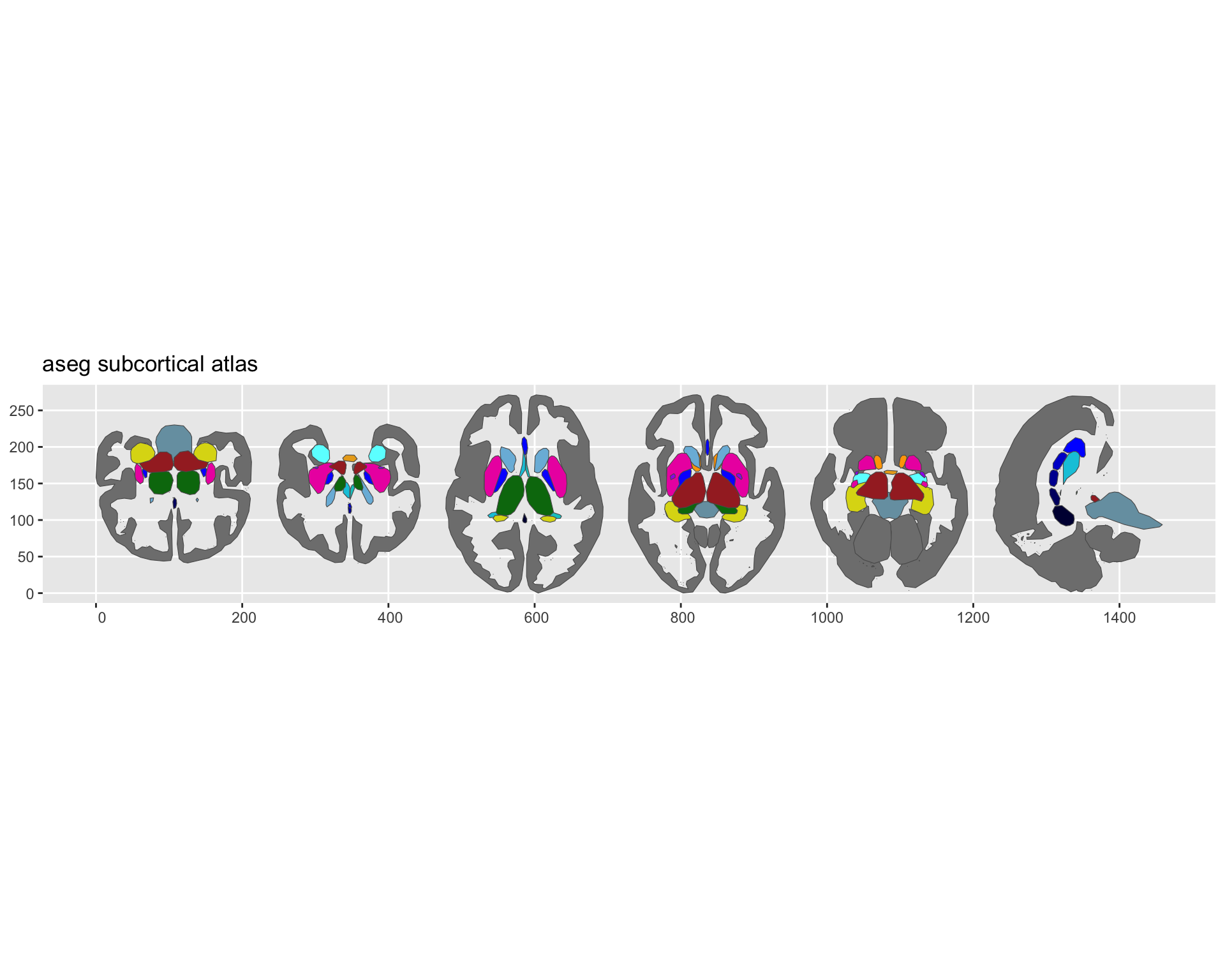
Subcortical aseg atlas plotted with ggseg.
Atlases not in FreeSurfer space
aseg is already on the FreeSurfer grid, so its structures sit in anatomical context for free. An atlas that ships as a standalone parcellation volume (in MNI space, say) has no surrounding brain to draw. prepare_subcortical_anatomical() coregisters such a parcellation to a FreeSurfer subject and merges it with that subject’s aparc+aseg, so the pipeline can draw the cortical ribbon and white-matter interior as context:
merged <- prepare_subcortical_anatomical(
  input_volume = "my_parcellation_2mm.nii.gz",
  lut = my_lut, # its idx selects + names the labels to keep
  target_subject = "cvs_avg35_inMNI152" # subject to borrow context from
)

atlas <- create_subcortical_from_volume(
  input_volume = merged, # carries both volume and matching colour table
  context = list(focus = "my-structures")
)
It chains coregister_volume() (wrapping mri_coreg to produce a reusable LTA transform) and project_volume_anatomical() (which resamples each label, takes the per-voxel argmax, shifts the atlas ids clear of the FreeSurfer ones, and protects the cortex). The result is a list(volume, lut, id_offset): the merged volume and a colour table aligned to it — FreeSurfer names for the aparc+aseg context labels plus your atlas labels at their shifted ids. create_subcortical_from_volume() unpacks both, so the context regions render with names aseg_context() recognises. Call the two steps separately to reuse one transform across several parcellations.
Custom colour tables
When an atlas adds labels FreeSurfer doesn’t know about, lut_add() appends them to a colour table; lut_combine() merges several tables and warns on clashing indices. Build my_lut from your parcellation’s own labels before passing it as lut above — prepare_subcortical_anatomical() shifts it and folds in the FreeSurfer context names for you: