Tract atlases represent white matter pathways derived from diffusion MRI tractography. Unlike cortical or subcortical atlases where regions are contiguous surfaces, tracts are tube-like structures that follow streamline bundles through the brain.
The pipeline reads tractography files, computes a centerline for each tract, wraps it in a tube mesh, and (optionally) creates 2D projection views.
This tutorial recreates the TRACULA atlas — the same pipeline behind data-raw/make_tracula_atlas.R in ggseg.formats.
What you need
- FreeSurfer installed with TRACULA training data (
trctrain/) - ImageMagick for 2D geometry extraction
- Chrome/Chromium for 3D screenshots
Finding tractography files
TRACULA training data ships with FreeSurfer in the trctrain/ directory. Each .trk file contains streamlines for one tract:
fs_dir <- freesurfer::fs_dir()
tract_dir <- file.path(fs_dir, "trctrain", "hcp", "mgh_1017", "mni")

tract_files <- list.files(tract_dir, pattern = "\\.trk$", full.names = TRUE)
aseg_file <- file.path(tract_dir, "aparc+aseg.nii.gz")

length(tract_files)
#> [1] 42
The aparc+aseg.nii.gz provides cortex outlines for 2D projections. If it’s missing, you can still create a 3D-only atlas.
Creating the atlas
create_tract_from_tractography() reads each tractography file, computes a centerline, and generates a tube mesh around it. The input_aseg provides cortex context for 2D views:
tracula_raw <- create_tract_from_tractography(
  input_tracts = tract_files,
  input_aseg = aseg_file,
  atlas_name = "tracula"
)
#> Warning: Atlas has 11230 vertices (threshold:
#> 10000)
#> ℹ Large atlases may be slow to plot and
#>   increase package size
#> ℹ Call `atlas_smooth(atlas, keep = 0.2,
#>   exclude = "cortex_")` to reduce vertices

tracula_raw
#>
#> ── tracts ggseg atlas ────────────────────
#> Type: tract
#> Regions: 26
#> Hemispheres: midline, left, right
#> Views: axial_1, axial_2, axial_3,
#> axial_4, axial_5, coronal_1, coronal_2,
#> coronal_3, coronal_4, coronal_5,
#> coronal_6, sagittal_left,
#> sagittal_midline, sagittal_right
#> Palette: ✖
#> Rendering: ✔ ggseg
#> ✔ ggseg3d (centerlines)
#> ──────────────────────────────────────────
#> # A tibble: 42 × 3
#>    hemi    region               label
#>    <chr>   <chr>                <chr>
#>  1 midline acomm.bbr.prep       acomm.bbr…
#>  2 midline cc.bodyc.bbr.prep    cc.bodyc.…
#>  3 midline cc.bodyp.bbr.prep    cc.bodyp.…
#>  4 midline cc.bodypf.bbr.prep   cc.bodypf…
#>  5 midline cc.bodypm.bbr.prep   cc.bodypm…
#>  6 midline cc.bodyt.bbr.prep    cc.bodyt.…
#>  7 midline cc.genu.bbr.prep     cc.genu.b…
#>  8 midline cc.rostrum.bbr.prep  cc.rostru…
#>  9 midline cc.splenium.bbr.prep cc.spleni…
#> 10 left    af.bbr.prep          lh.af.bbr…
#> 11 left    ar.bbr.prep          lh.ar.bbr…
#> 12 left    atr.bbr.prep         lh.atr.bb…
#> 13 left    cbd.bbr.prep         lh.cbd.bb…
#> 14 left    cbv.bbr.prep         lh.cbv.bb…
#> 15 left    cst.bbr.prep         lh.cst.bb…
#> 16 left    emc.bbr.prep         lh.emc.bb…
#> 17 left    fat.bbr.prep         lh.fat.bb…
#> 18 left    fx.bbr.prep          lh.fx.bbr…
#> 19 left    ilf.bbr.prep         lh.ilf.bb…
#> 20 left    mlf.bbr.prep         lh.mlf.bb…
#> 21 left    or.bbr.prep          lh.or.bbr…
#> 22 left    slf1.bbr.prep        lh.slf1.b…
#> 23 left    slf2.bbr.prep        lh.slf2.b…
#> 24 left    slf3.bbr.prep        lh.slf3.b…
#> 25 left    uf.bbr.prep          lh.uf.bbr…
#> 26 midline mcp.bbr.prep         mcp.bbr.p…
#> 27 right   af.bbr.prep          rh.af.bbr…
#> 28 right   ar.bbr.prep          rh.ar.bbr…
#> 29 right   atr.bbr.prep         rh.atr.bb…
#> 30 right   cbd.bbr.prep         rh.cbd.bb…
#> 31 right   cbv.bbr.prep         rh.cbv.bb…
#> 32 right   cst.bbr.prep         rh.cst.bb…
#> 33 right   emc.bbr.prep         rh.emc.bb…
#> 34 right   fat.bbr.prep         rh.fat.bb…
#> 35 right   fx.bbr.prep          rh.fx.bbr…
#> 36 right   ilf.bbr.prep         rh.ilf.bb…
#> 37 right   mlf.bbr.prep         rh.mlf.bb…
#> 38 right   or.bbr.prep          rh.or.bbr…
#> 39 right   slf1.bbr.prep        rh.slf1.b…
#> 40 right   slf2.bbr.prep        rh.slf2.b…
#> 41 right   slf3.bbr.prep        rh.slf3.b…
#> 42 right   uf.bbr.prep          rh.uf.bbr…
Key parameters:
-
tube_radiuscontrols tube thickness. Larger values make tracts more visible at the cost of anatomical precision. -
tube_segmentscontrols the number of vertices around the tube circumference. Six gives hexagonal cross-sections; 12+ gives smoother tubes. -
n_pointscontrols centerline resolution. More points capture finer curvature.
Post-processing
Selecting views
Keep the projections that show your tracts best:
tracula_raw <- tracula_raw |>
  atlas_view_keep(c(
    "axial_2",
    "axial_4",
    "coronal_3",
    "coronal_4",
    "sagittal"
  ))
Setting context regions
Add cortex as a background outline:
tracula_raw <- tracula_raw |>
  atlas_region_contextual("cortex")
Removing small fragments
After view selection, some tracts may appear as tiny slivers in certain views. Remove fragments below a minimum area:
tracula_raw <- tracula_raw |>
  atlas_view_remove_small(
    min_area = 500,
    views = c("axial", "coronal")
  ) |>
  atlas_view_remove_small(min_area = 50)
#> ℹ Removed 49 geometries below area 500
#> ℹ Removed 10 geometries below area 50
The first call applies a higher threshold to axial and coronal views (where tracts appear in cross-section and produce small dots). The second call applies a lower threshold everywhere to catch remaining slivers.
Adding metadata
Join tract group information — which tracts are projection fibres, which are commissural, which are association:
normalize_label <- function(x) {
  x |>
    basename() |>
    tools::file_path_sans_ext()
}

tracula_metadata <- data.frame(
  label_key = c(
    "lh.cst.bbr.prep", "rh.cst.bbr.prep",
    "lh.ilf.bbr.prep", "rh.ilf.bbr.prep",
    "lh.unc.bbr.prep", "rh.unc.bbr.prep",
    "lh.atr.bbr.prep", "rh.atr.bbr.prep",
    "lh.cab.bbr.prep", "rh.cab.bbr.prep",
    "lh.slfp.bbr.prep", "rh.slfp.bbr.prep",
    "lh.slft.bbr.prep", "rh.slft.bbr.prep",
    "lh.ccg.bbr.prep", "rh.ccg.bbr.prep",
    "fmajor.bbr.prep", "fminor.bbr.prep"
  ),
  region = c(
    "corticospinal tract", "corticospinal tract",
    "inferior longitudinal fasciculus", "inferior longitudinal fasciculus",
    "uncinate fasciculus", "uncinate fasciculus",
    "anterior thalamic radiation", "anterior thalamic radiation",
    "cingulum (angular bundle)", "cingulum (angular bundle)",
    "SLF (parietal)", "SLF (parietal)",
    "SLF (temporal)", "SLF (temporal)",
    "cingulum (cingulate gyrus)", "cingulum (cingulate gyrus)",
    "forceps major", "forceps minor"
  ),
  group = c(
    "projection", "projection",
    "association", "association",
    "association", "association",
    "projection", "projection",
    "limbic", "limbic",
    "association", "association",
    "association", "association",
    "limbic", "limbic",
    "commissural", "commissural"
  )
)

core_with_meta <- tracula_raw$core |>
  mutate(label_key = normalize_label(label)) |>
  left_join(
    tracula_metadata |> select(label_key, region_pretty = region, group),
    by = "label_key"
  ) |>
  mutate(region = coalesce(region_pretty, region)) |>
  select(hemi, region, label, group)
Rebuilding and saving
tracula <- ggseg_atlas(
  atlas = "tracula",
  type = "tract",
  palette = tracula_raw$palette,
  core = core_with_meta,
  data = tracula_raw$data
)

tracula
#>
#> ── tracula ggseg atlas ───────────────────
#> Type: tract
#> Regions: 26
#> Hemispheres: midline, left, right
#> Views: axial_2, axial_4, coronal_3,
#> coronal_4, sagittal_left,
#> sagittal_midline, sagittal_right
#> Palette: ✖
#> Rendering: ✔ ggseg
#> ✔ ggseg3d (centerlines)
#> ──────────────────────────────────────────
#> # A tibble: 42 × 4
#>    hemi    region              label group
#>    <chr>   <chr>               <chr> <chr>
#>  1 midline acomm.bbr.prep      acom… <NA>
#>  2 midline cc.bodyc.bbr.prep   cc.b… <NA>
#>  3 midline cc.bodyp.bbr.prep   cc.b… <NA>
#>  4 midline cc.bodypf.bbr.prep  cc.b… <NA>
#>  5 midline cc.bodypm.bbr.prep  cc.b… <NA>
#>  6 midline cc.bodyt.bbr.prep   cc.b… <NA>
#>  7 midline cc.genu.bbr.prep    cc.g… <NA>
#>  8 midline cc.rostrum.bbr.prep cc.r… <NA>
#>  9 midline cc.splenium.bbr.pr… cc.s… <NA>
#> 10 left    af.bbr.prep         lh.a… <NA>
#> 11 left    ar.bbr.prep         lh.a… <NA>
#> 12 left    atr.bbr.prep        lh.a… <NA>
#> 13 left    cbd.bbr.prep        lh.c… <NA>
#> 14 left    cbv.bbr.prep        lh.c… <NA>
#> 15 left    cst.bbr.prep        lh.c… <NA>
#> 16 left    emc.bbr.prep        lh.e… <NA>
#> 17 left    fat.bbr.prep        lh.f… <NA>
#> 18 left    fx.bbr.prep         lh.f… <NA>
#> 19 left    ilf.bbr.prep        lh.i… <NA>
#> 20 left    mlf.bbr.prep        lh.m… <NA>
#> 21 left    or.bbr.prep         lh.o… <NA>
#> 22 left    slf1.bbr.prep       lh.s… <NA>
#> 23 left    slf2.bbr.prep       lh.s… <NA>
#> 24 left    slf3.bbr.prep       lh.s… <NA>
#> 25 left    uf.bbr.prep         lh.u… <NA>
#> 26 midline mcp.bbr.prep        mcp.… <NA>
#> 27 right   af.bbr.prep         rh.a… <NA>
#> 28 right   ar.bbr.prep         rh.a… <NA>
#> 29 right   atr.bbr.prep        rh.a… <NA>
#> 30 right   cbd.bbr.prep        rh.c… <NA>
#> 31 right   cbv.bbr.prep        rh.c… <NA>
#> 32 right   cst.bbr.prep        rh.c… <NA>
#> 33 right   emc.bbr.prep        rh.e… <NA>
#> 34 right   fat.bbr.prep        rh.f… <NA>
#> 35 right   fx.bbr.prep         rh.f… <NA>
#> 36 right   ilf.bbr.prep        rh.i… <NA>
#> 37 right   mlf.bbr.prep        rh.m… <NA>
#> 38 right   or.bbr.prep         rh.o… <NA>
#> 39 right   slf1.bbr.prep       rh.s… <NA>
#> 40 right   slf2.bbr.prep       rh.s… <NA>
#> 41 right   slf3.bbr.prep       rh.s… <NA>
#> 42 right   uf.bbr.prep         rh.u… <NA>
atlas_labels(tracula)
#>  [1] "acomm.bbr.prep"
#>  [2] "cc.bodyc.bbr.prep"
#>  [3] "cc.bodyp.bbr.prep"
#>  [4] "cc.bodypf.bbr.prep"
#>  [5] "cc.bodypm.bbr.prep"
#>  [6] "cc.bodyt.bbr.prep"
#>  [7] "cc.genu.bbr.prep"
#>  [8] "cc.rostrum.bbr.prep"
#>  [9] "cc.splenium.bbr.prep"
#> [10] "lh.af.bbr.prep"
#> [11] "lh.ar.bbr.prep"
#> [12] "lh.atr.bbr.prep"
#> [13] "lh.cbd.bbr.prep"
#> [14] "lh.cbv.bbr.prep"
#> [15] "lh.cst.bbr.prep"
#> [16] "lh.emc.bbr.prep"
#> [17] "lh.fat.bbr.prep"
#> [18] "lh.fx.bbr.prep"
#> [19] "lh.ilf.bbr.prep"
#> [20] "lh.mlf.bbr.prep"
#> [21] "lh.or.bbr.prep"
#> [22] "lh.slf1.bbr.prep"
#> [23] "lh.slf2.bbr.prep"
#> [24] "lh.slf3.bbr.prep"
#> [25] "lh.uf.bbr.prep"
#> [26] "mcp.bbr.prep"
#> [27] "rh.af.bbr.prep"
#> [28] "rh.ar.bbr.prep"
#> [29] "rh.atr.bbr.prep"
#> [30] "rh.cbd.bbr.prep"
#> [31] "rh.cbv.bbr.prep"
#> [32] "rh.cst.bbr.prep"
#> [33] "rh.emc.bbr.prep"
#> [34] "rh.fat.bbr.prep"
#> [35] "rh.fx.bbr.prep"
#> [36] "rh.ilf.bbr.prep"
#> [37] "rh.mlf.bbr.prep"
#> [38] "rh.or.bbr.prep"
#> [39] "rh.slf1.bbr.prep"
#> [40] "rh.slf2.bbr.prep"
#> [41] "rh.slf3.bbr.prep"
#> [42] "rh.uf.bbr.prep"

table(tracula$core$group, useNA = "ifany")
#>
#> <NA>
#>   42
plot(tracula) +
  ggplot2::scale_fill_viridis_d(na.value = "grey80")
#> Scale for fill is already present.
#> Adding another scale for fill, which will
#> replace the existing scale.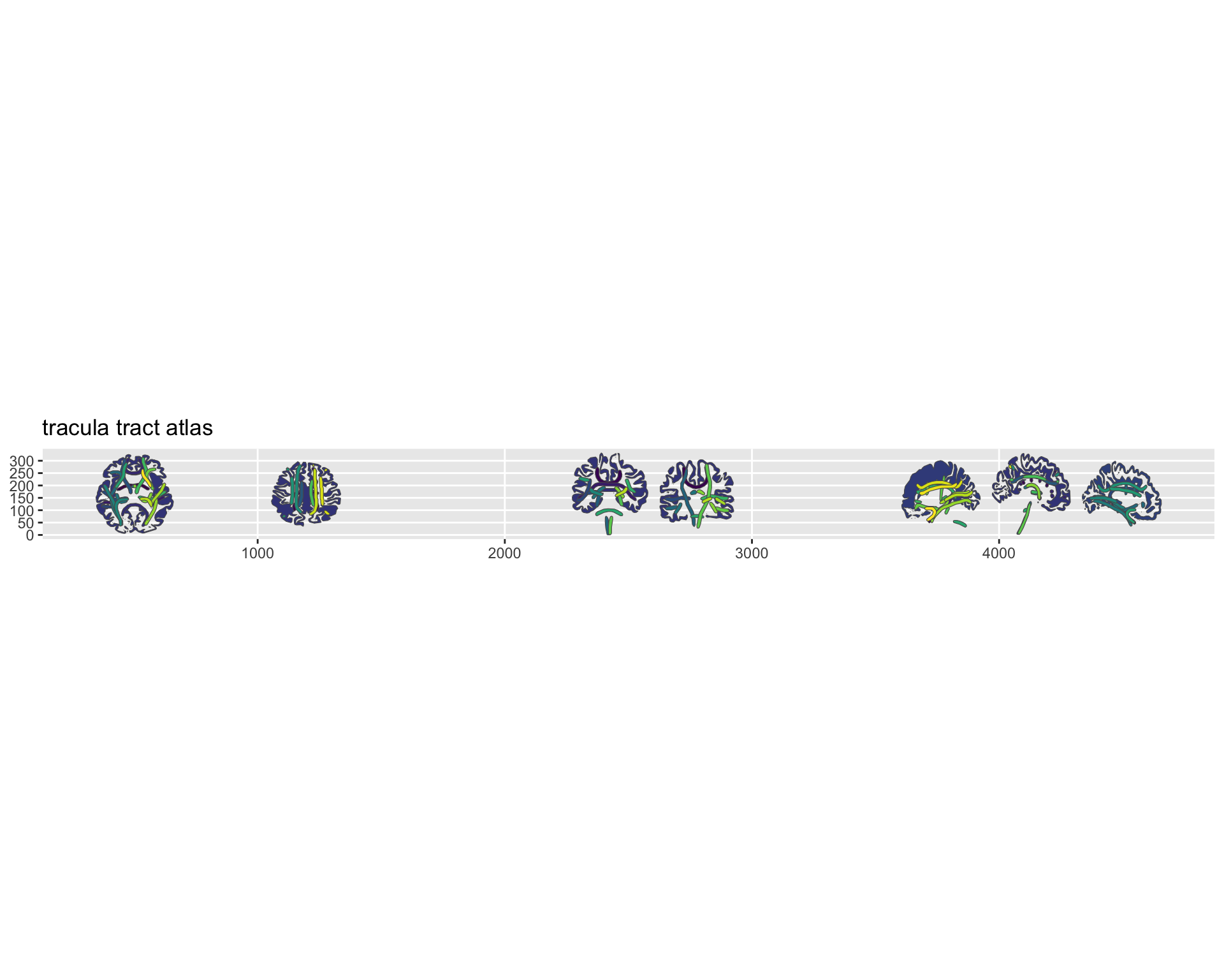
TRACULA white matter tract atlas plotted with ggseg.