
Placing points and combining atlases
Source:vignettes/articles/point-placement.Rmd
point-placement.RmdSooner or later you want something on the brain that is not a
parcellation: electrode positions, a stimulation target, the peak of a
cluster. add_points() draws those, and
add_atlas() puts a second atlas in the same scene.
The drawing is the easy part. The part worth reading about is which coordinates to give them, because a plausible-looking number in the wrong space produces a plausible-looking picture that is wrong.
Points need a surface that means something
Every ggseg3d cortical surface is fsaverage5, but they are not
interchangeable. "white" and "pial" keep the
brain’s own shape. "inflated" — what ggseg3d()
draws by default — has had every vertex moved outward to smooth the
folds away.
Here is the same set of coordinates on both. They were taken straight off the pial surface, so they sit exactly on it:
pial <- resolve_brain_mesh("rh", "pial")$vertices
set.seed(7)
pts <- pial[sample(nrow(pial), 14), ]

ggseg3d(atlas = dk(), hemisphere = "right", surface = "pial") |>
  add_points(pts, x = x, y = y, z = z, colour = "#111111", size = 4) |>
  pan_camera("right lateral")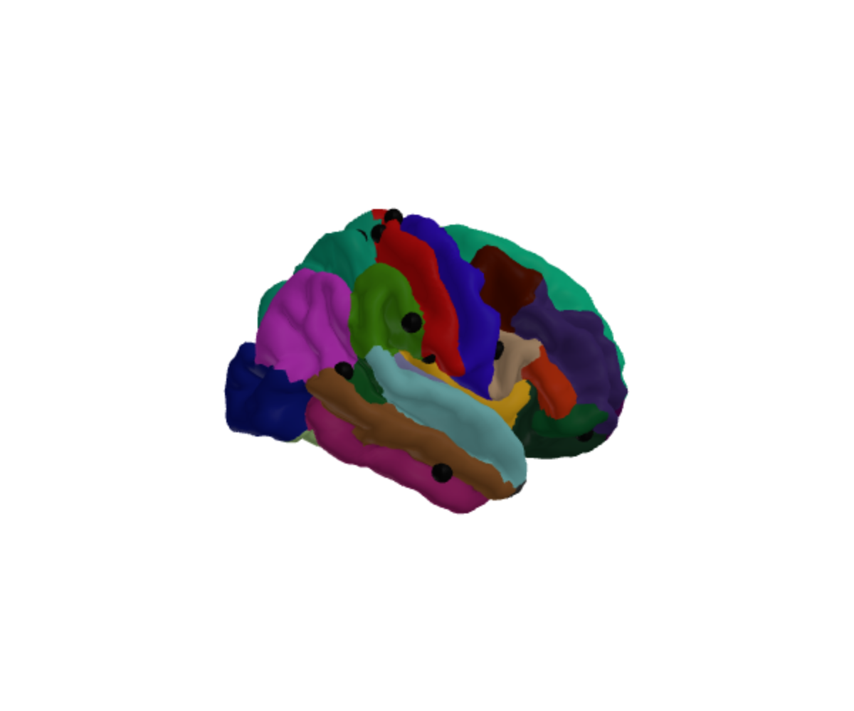
Change nothing but the surface and most of them disappear inside the brain:
ggseg3d(atlas = dk(), hemisphere = "right", surface = "inflated") |>
  add_points(pts, x = x, y = y, z = z, colour = "#111111", size = 4) |>
  pan_camera("right lateral")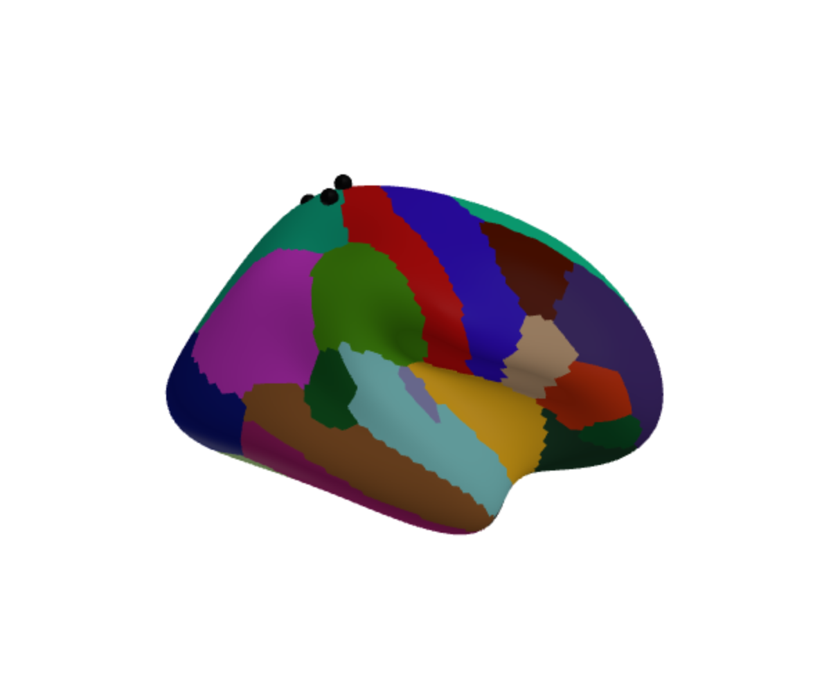
Nothing went wrong in either plot. The inflated surface is simply a
different shape, so a position on the real brain is not a position on
it. Plot measured coordinates on "pial" or
"white".
Getting coordinates from a standard space
If your positions come from somewhere else — a montage file, a
coordinate table, a paper — they are probably in MNI.
mni_to_mesh() converts them:
mni_to_mesh(-42, -20, 55, hemisphere = "lh")## x y z
## 1 -43.22156 -20 55The shift is small because the surfaces nearly are MNI
already. fsaverage is an MNI305 average, so its coordinates are MNI305;
the only difference is that each hemisphere is nudged sideways so the
two meet at x = 0 and can be drawn together.
mesh_to_mni() undoes that.
Pass space = "mni152" if your coordinates are MNI152
rather than MNI305. Across the brain that is worth two to three
millimetres:
rbind(
  mni305 = mni_to_mesh(-42, -20, 55, hemisphere = "lh"),
  mni152 = mni_to_mesh(-42, -20, 55, hemisphere = "lh", space = "mni152")
)
## x y z
## mni305 -43.22156 -20.00000 55.00000
## mni152 -44.37479 -20.77315 53.21614Asking for an inflated surface is an error rather than a number, because there is no honest answer:
mesh_to_mni(-42, -20, 55, hemisphere = "lh", surface = "inflated")## Error in `mesh_to_mni()`:
## ! "inflated" has no anatomical coordinates to convert.
## ✖ Inflation and spherical registration move every vertex, so a position on this
## surface does not correspond to a place in the brain.
## ℹ Use one of "white", "pial", "midthickness", "smoothwm", and "orig".A worked example
Three motor-cortex coordinates:
targets <- data.frame(
  label = c("M1 hand", "M1 face", "SMA"),
  x = c(-38, -52, -4),
  y = c(-22, -8, -4),
  z = c(56, 34, 58)
)

placed <- mni_to_mesh(targets$x, targets$y, targets$z, hemisphere = "lh")
placed$label <- targets$label
placed
## x y z label
## 1 -39.221563 -22 56 M1 hand
## 2 -53.221563 -8 34 M1 face
## 3 -5.221563 -4 58 SMADraw those directly and you will see nothing at all, which is worth understanding rather than working around. A coordinate reported as a peak is a point in grey matter, a millimetre or two beneath the surface — so the marker is there, with the cortex in front of it. That is the opposite of the earlier failure: these are in exactly the right place, and still invisible.
Either make the marker big enough to break the surface, or put it on the surface. Projecting to the nearest vertex is a few lines and keeps the position honest:
pial <- resolve_brain_mesh("lh", "pial")$vertices

on_surface <- do.call(rbind, lapply(seq_len(nrow(placed)), function(i) {
  d2 <- (pial$x - placed$x[i])^2 +
    (pial$y - placed$y[i])^2 +
    (pial$z - placed$z[i])^2
  pial[which.min(d2), ]
}))
on_surface$label <- placed$label
This one is live: drag to rotate, and hover a marker for its name.
ggseg3d(atlas = dk(), hemisphere = "left", surface = "pial") |>
  add_points(on_surface, x = x, y = y, z = z, text = label,
             colour = "#D7191C", size = 4) |>
  pan_camera("left lateral")
colour and size take one value or one per
row, so a column of values can drive either.
Two atlases at once
add_atlas() draws another atlas into the same scene —
subcortical structures inside a cortical surface, say:
ggseg3d(atlas = dk(), hemisphere = "left") |>
  add_atlas(aseg()) |>
  pan_camera("right lateral")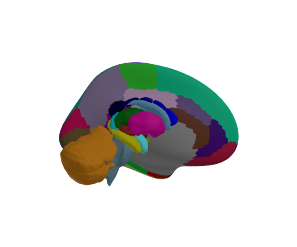
Or the other way round, with the cortex as a translucent shell:
ggseg3d(atlas = aseg()) |>
  add_glassbrain(opacity = 0.12) |>
  pan_camera("right lateral")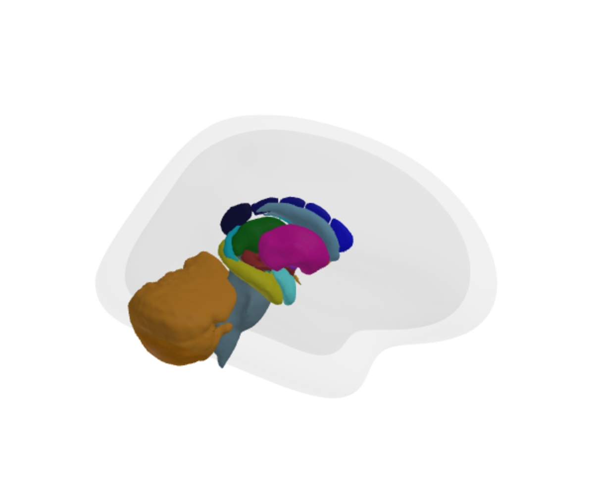
Two things to know.
The atlases are not registered against each other.
They line up because the ggsegverse atlases share an anatomical frame,
not because add_atlas() reconciles them. If you bring your
own atlas from elsewhere, check that it agrees before trusting the
overlap.
And the legend describes the atlas the plot was built from, not the one added. If the second atlas needs a readable legend, build the plot from that one and add the other.
Why the cerebellum sticks out
In the picture above the cerebellum extends past the glass brain. That is anatomically right — the cerebellum is not inside the cerebral cortex — but the default glass brain is the inflated surface, which is larger and rounder than any real brain. For judging whether something sits inside the cortex, use an anatomical shell:
ggseg3d(atlas = aseg()) |>
  add_glassbrain(surface = "white", opacity = 0.15)
In short
- Measured coordinates belong on
"pial"or"white", never"inflated". -
mni_to_mesh()gets you there from MNI305 or MNI152. - A peak coordinate sits inside the cortex; project it to the surface, or enlarge the marker, if you expect to see it.
-
add_atlas()composes atlases that already share a frame; it does not create one.