geom_brain() handles data joining and positioning
automatically, which covers most use cases. But because it owns the data
pipeline, you can’t easily layer other sf geoms on top – things like
geom_sf_label() or geom_sf_text() need direct
access to the sf data.
This vignette shows how to work with brain atlases as plain sf objects, giving you full control at the cost of a few extra lines.
This is the one workflow that needs the sf package,
which ggseg now treats as an optional dependency. Install it with
install.packages("sf") if you don’t already have it.
Everywhere else, geom_brain() plots the same atlases
without sf.
library(ggseg)
library(ggplot2)
library(dplyr)
#>
#> Attaching package: 'dplyr'
#> The following objects are masked from 'package:stats':
#>
#>     filter, lag
#> The following objects are masked from 'package:base':
#>
#>     intersect, setdiff, setequal, union
When you’d want this
Use the sf workflow when you need to:
- Add region labels with
geom_sf_label()orgeom_sf_text() - Use
ggrepel::geom_label_repel()for non-overlapping labels - Layer other sf geoms on the brain
- Have full control over the data before it reaches ggplot
For everything else, geom_brain() is simpler.
Getting atlas data as sf
A brain atlas stores its geometry in the data slot.
Convert to a plain data frame to see all the columns:
dk()$data
#>
#> ── ggseg_data_cortical ──
#>
#> 2D (ggseg): 72 labels (polygons), views: inferior, lateral, superior, medial
#> 3D (ggseg3d): vertex indices
#>                         label    vertices
#> 1                 lh_bankssts <int [126]>
#> 2  lh_caudalanteriorcingulate  <int [67]>
#> 3      lh_caudalmiddlefrontal <int [232]>
#> 4           lh_corpuscallosum <int [198]>
#> 5                   lh_cuneus <int [102]>
#> 6               lh_entorhinal  <int [48]>
#> 7                 lh_fusiform <int [308]>
#> 8         lh_inferiorparietal <int [484]>
#> 9         lh_inferiortemporal <int [271]>
#> 10        lh_isthmuscingulate <int [123]>
#> ... with 60 more rows
The geometry column holds the polygons. This is a
standard sf object, so any sf-compatible tool works with it.
Joining your data
Use brain_join() to merge your data with the atlas. It
preserves the sf geometry and handles column detection:
some_data <- tibble(
  region = c(
    "transverse temporal",
    "insula",
    "precentral",
    "superior parietal"
  ),
  p = sample(seq(0, 0.5, 0.001), 4)
)

some_data |>
  brain_join(dk())
#> Merging atlas and data by region.
#> Simple feature collection with 191 features and 9 fields
#> Geometry type: MULTIPOLYGON
#> Dimension:     XY
#> Bounding box:  xmin: 84.2049 ymin: 0 xmax: 5359.689 ymax: 429.9372
#> CRS:           NA
#> First 10 features:
#>                         label     view  hemi                            region
#> 1                  lh_unknown  lateral  left                              <NA>
#> 2                  lh_unknown   medial  left                              <NA>
#> 3                  lh_unknown inferior  left                              <NA>
#> 4                  rh_unknown  lateral right                              <NA>
#> 5                  rh_unknown   medial right                              <NA>
#> 6                  rh_unknown inferior right                              <NA>
#> 7                 lh_bankssts  lateral  left banks of superior temporal sulcus
#> 8                 lh_bankssts superior  left banks of superior temporal sulcus
#> 9                 lh_bankssts inferior  left banks of superior temporal sulcus
#> 10 lh_caudalanteriorcingulate   medial  left         caudal anterior cingulate
#>         lobe atlas     type  colour  p                       geometry
#> 1       <NA>    dk cortical    <NA> NA MULTIPOLYGON (((926.5936 60...
#> 2       <NA>    dk cortical    <NA> NA MULTIPOLYGON (((1782.84 18....
#> 3       <NA>    dk cortical    <NA> NA MULTIPOLYGON (((367.1256 13...
#> 4       <NA>    dk cortical    <NA> NA MULTIPOLYGON (((3849.766 60...
#> 5       <NA>    dk cortical    <NA> NA MULTIPOLYGON (((4318.844 20...
#> 6       <NA>    dk cortical    <NA> NA MULTIPOLYGON (((3190.519 5....
#> 7   temporal    dk cortical #196428 NA MULTIPOLYGON (((1121.478 12...
#> 8   temporal    dk cortical #196428 NA MULTIPOLYGON (((2448.464 20...
#> 9   temporal    dk cortical #196428 NA MULTIPOLYGON (((534.4782 21...
#> 10 cingulate    dk cortical #7D64A0 NA MULTIPOLYGON (((1921.971 20...
The result is a standard sf object you can pass to
geom_sf().
Plotting with geom_sf
some_data |>
  brain_join(dk()) |>
  ggplot() +
  geom_sf(aes(fill = p))
#> Merging atlas and data by region.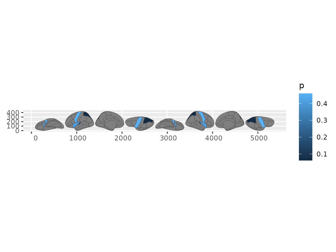
Brain plot using geom_sf after brain_join.
Repositioning views
With geom_brain(), you’d use
position_brain(). In the sf workflow, use
reposition_brain() instead – it transforms the geometry
directly:
some_data |>
  brain_join(dk()) |>
  reposition_brain(hemi ~ view) |>
  ggplot() +
  geom_sf(aes(fill = p))
#> Merging atlas and data by region.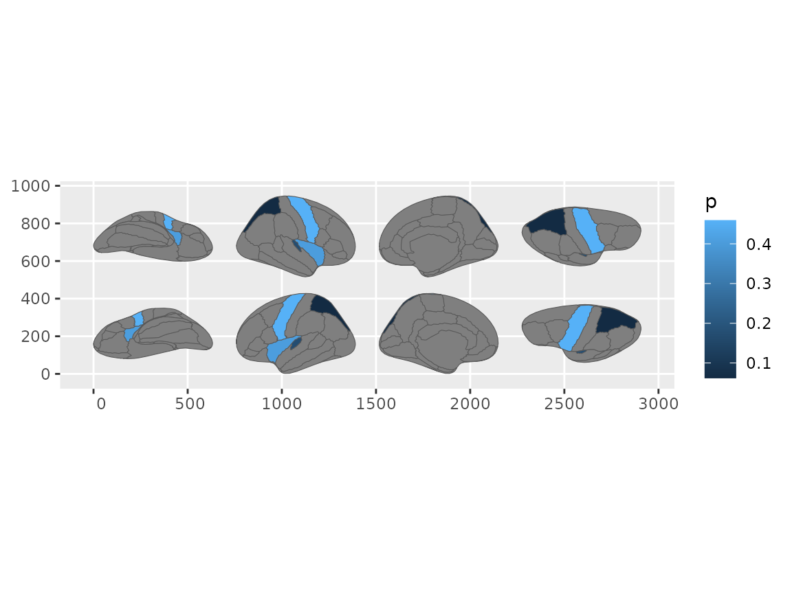
Repositioned brain views using reposition_brain() with geom_sf.
Same formula syntax, same results.
Adding labels
This is the main reason to use the sf workflow. Once you have repositioned sf data, you can layer any sf geom:
some_data |>
  brain_join(dk()) |>
  reposition_brain(hemi ~ view) |>
  ggplot(aes(fill = p)) +
  geom_sf(show.legend = FALSE) +
  geom_sf_label(
    aes(label = ifelse(!is.na(p), region, NA)),
    alpha = 0.8,
    show.legend = FALSE
  )
#> Merging atlas and data by region.
#> Warning: Removed 168 rows containing missing values or values outside the scale range
#> (`geom_label()`).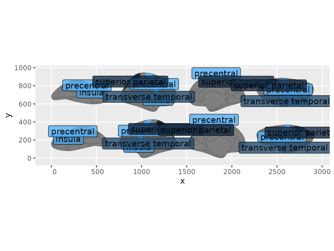
Brain regions with text labels overlaid using geom_sf_label.
For crowded plots, ggrepel::geom_label_repel() avoids
overlapping labels.
Faceting with grouped data
In the sf workflow, faceting requires group_by() before
brain_join(). The grouping tells the join to replicate the
atlas for each group:
some_data <- tibble(
  region = rep(
    c(
      "transverse temporal",
      "insula",
      "precentral",
      "superior parietal"
    ),
    2
  ),
  p = sample(seq(0, 0.5, 0.001), 8),
  group = c(rep("A", 4), rep("B", 4))
)

some_data |>
  group_by(group) |>
  brain_join(dk()) |>
  reposition_brain(hemi ~ view) |>
  ggplot(aes(fill = p)) +
  geom_sf(show.legend = FALSE) +
  facet_wrap(~group)
#> Merging atlas and data by region.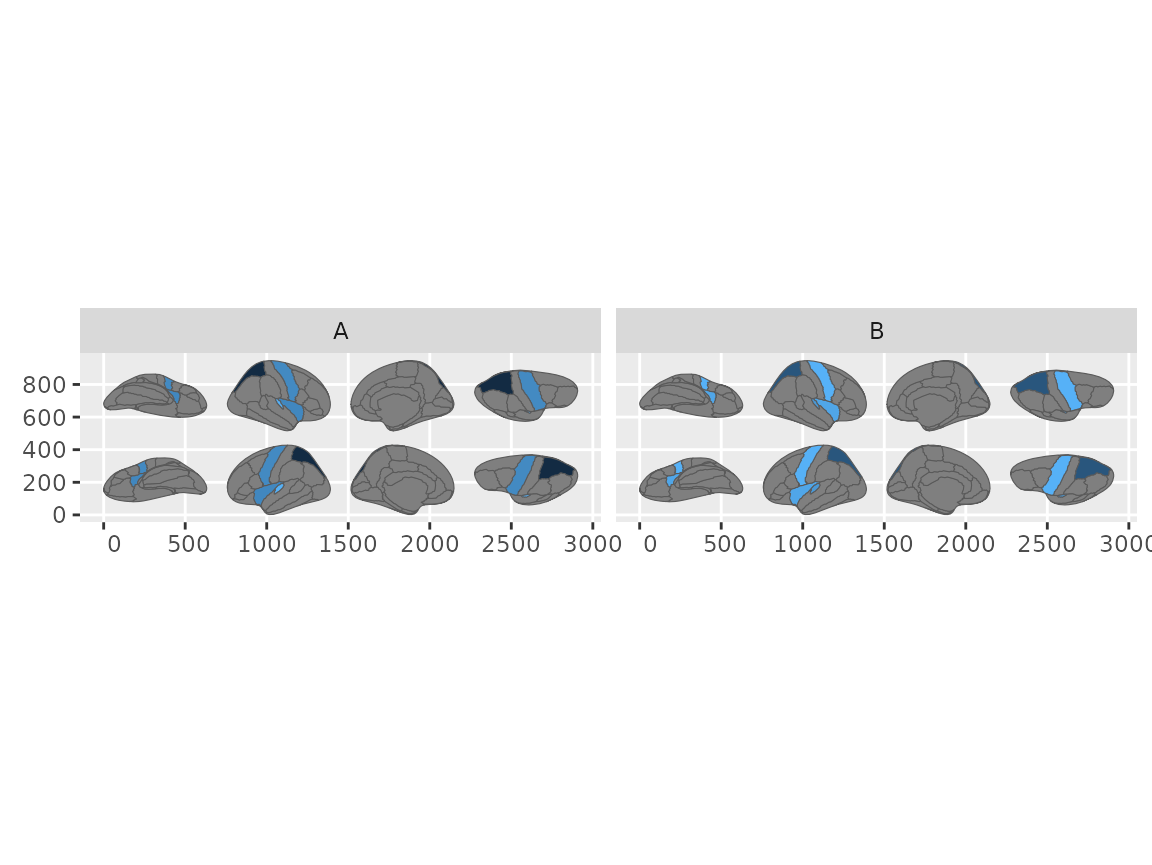
Faceted brain plots using the geom_sf workflow with grouped data.
This step is only needed in the sf workflow.
geom_brain() handles atlas replication automatically (see
vignette("external-data")).