If you work with neuroimaging data, you’ve probably spent time wrestling region-level results into brain plots. ggseg handles that plumbing for you. It stores brain atlas geometries and plots them as ggplot2 layers, so you get brain figures with the same code you’d use for any other ggplot.
What’s in a brain atlas
A brain_atlas object bundles four things: a name, a type
(cortical, subcortical, or tract), region geometry, and an optional
colour palette.
dk()
#>
#> ── dk ggseg atlas ──────────────────────────────────────────────────────────────
#> Type: cortical
#> Regions: 35
#> Hemispheres: left, right
#> Views: inferior, lateral, superior, medial
#> Palette: ✔
#> Rendering: ✔ ggseg
#> ✔ ggseg3d (vertices)
#> ────────────────────────────────────────────────────────────────────────────────
#>    hemi                            region                      label
#> 1  left banks of superior temporal sulcus                lh_bankssts
#> 2  left         caudal anterior cingulate lh_caudalanteriorcingulate
#> 3  left             caudal middle frontal     lh_caudalmiddlefrontal
#> 4  left                   corpus callosum          lh_corpuscallosum
#> 5  left                            cuneus                  lh_cuneus
#> 6  left                        entorhinal              lh_entorhinal
#> 7  left                          fusiform                lh_fusiform
#> 8  left                 inferior parietal        lh_inferiorparietal
#> 9  left                 inferior temporal        lh_inferiortemporal
#> 10 left                 isthmus cingulate        lh_isthmuscingulate
#>            lobe
#> 1      temporal
#> 2     cingulate
#> 3       frontal
#> 4  white matter
#> 5     occipital
#> 6      temporal
#> 7      temporal
#> 8      parietal
#> 9      temporal
#> 10    cingulate
#> ... with 60 more rows
The dk atlas (Desikan-Killiany) ships with the package.
Call plot() for a quick look:
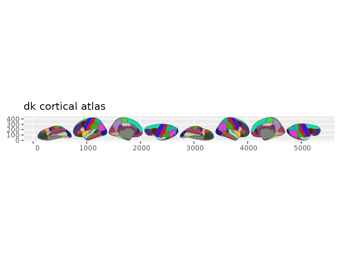
Quick overview of the Desikan-Killiany cortical atlas.
Two helpers pull out the names you’ll need for matching data:
library(ggseg.formats)

atlas_regions(dk())
#>  [1] "banks of superior temporal sulcus" "caudal anterior cingulate"
#>  [3] "caudal middle frontal"             "corpus callosum"
#>  [5] "cuneus"                            "entorhinal"
#>  [7] "frontal pole"                      "fusiform"
#>  [9] "inferior parietal"                 "inferior temporal"
#> [11] "insula"                            "isthmus cingulate"
#> [13] "lateral occipital"                 "lateral orbitofrontal"
#> [15] "lingual"                           "medial orbitofrontal"
#> [17] "middle temporal"                   "paracentral"
#> [19] "parahippocampal"                   "pars opercularis"
#> [21] "pars orbitalis"                    "pars triangularis"
#> [23] "pericalcarine"                     "postcentral"
#> [25] "posterior cingulate"               "precentral"
#> [27] "precuneus"                         "rostral anterior cingulate"
#> [29] "rostral middle frontal"            "superior frontal"
#> [31] "superior parietal"                 "superior temporal"
#> [33] "supramarginal"                     "temporal pole"
#> [35] "transverse temporal"
atlas_labels(dk())
#>  [1] "lh_bankssts"                 "lh_caudalanteriorcingulate"
#>  [3] "lh_caudalmiddlefrontal"      "lh_corpuscallosum"
#>  [5] "lh_cuneus"                   "lh_entorhinal"
#>  [7] "lh_frontalpole"              "lh_fusiform"
#>  [9] "lh_inferiorparietal"         "lh_inferiortemporal"
#> [11] "lh_insula"                   "lh_isthmuscingulate"
#> [13] "lh_lateraloccipital"         "lh_lateralorbitofrontal"
#> [15] "lh_lingual"                  "lh_medialorbitofrontal"
#> [17] "lh_middletemporal"           "lh_paracentral"
#> [19] "lh_parahippocampal"          "lh_parsopercularis"
#> [21] "lh_parsorbitalis"            "lh_parstriangularis"
#> [23] "lh_pericalcarine"            "lh_postcentral"
#> [25] "lh_posteriorcingulate"       "lh_precentral"
#> [27] "lh_precuneus"                "lh_rostralanteriorcingulate"
#> [29] "lh_rostralmiddlefrontal"     "lh_superiorfrontal"
#> [31] "lh_superiorparietal"         "lh_superiortemporal"
#> [33] "lh_supramarginal"            "lh_temporalpole"
#> [35] "lh_transversetemporal"       "rh_bankssts"
#> [37] "rh_caudalanteriorcingulate"  "rh_caudalmiddlefrontal"
#> [39] "rh_corpuscallosum"           "rh_cuneus"
#> [41] "rh_entorhinal"               "rh_frontalpole"
#> [43] "rh_fusiform"                 "rh_inferiorparietal"
#> [45] "rh_inferiortemporal"         "rh_insula"
#> [47] "rh_isthmuscingulate"         "rh_lateraloccipital"
#> [49] "rh_lateralorbitofrontal"     "rh_lingual"
#> [51] "rh_medialorbitofrontal"      "rh_middletemporal"
#> [53] "rh_paracentral"              "rh_parahippocampal"
#> [55] "rh_parsopercularis"          "rh_parsorbitalis"
#> [57] "rh_parstriangularis"         "rh_pericalcarine"
#> [59] "rh_postcentral"              "rh_posteriorcingulate"
#> [61] "rh_precentral"               "rh_precuneus"
#> [63] "rh_rostralanteriorcingulate" "rh_rostralmiddlefrontal"
#> [65] "rh_superiorfrontal"          "rh_superiorparietal"
#> [67] "rh_superiortemporal"         "rh_supramarginal"
#> [69] "rh_temporalpole"             "rh_transversetemporal"
Your first brain plot
geom_brain() works like any ggplot2 geom. Pass it an
atlas and it draws the regions:
ggplot() +
  geom_brain(atlas = dk(), show.legend = FALSE)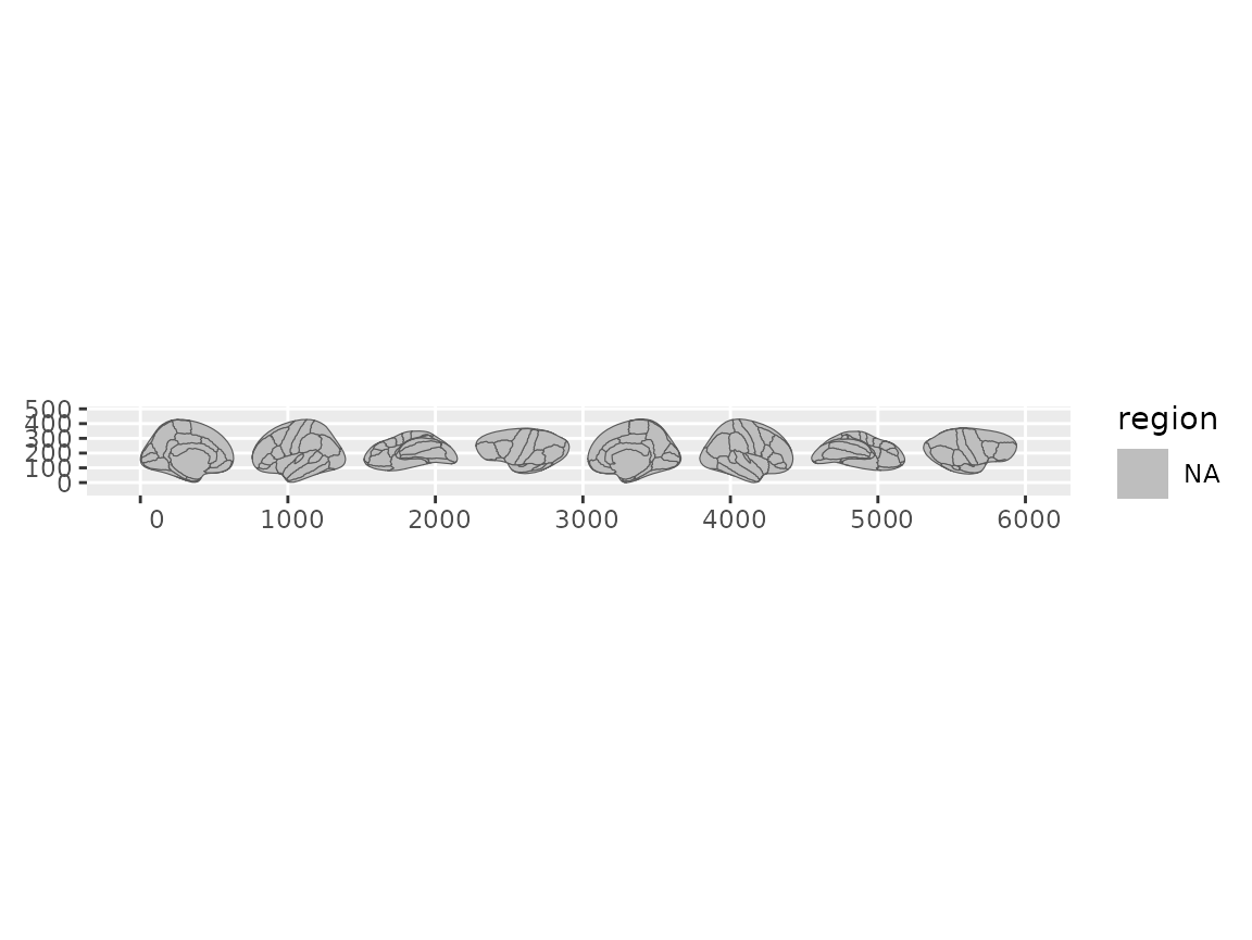
Default brain plot using geom_brain() with the dk atlas.
Arranging views
Brain atlases have multiple views (lateral, medial) and hemispheres.
position_brain() controls how they’re laid out, using
formula syntax borrowed from facet_grid():
ggplot() +
  geom_brain(
    atlas = dk(),
    position = position_brain(hemi ~ view),
    show.legend = FALSE
  )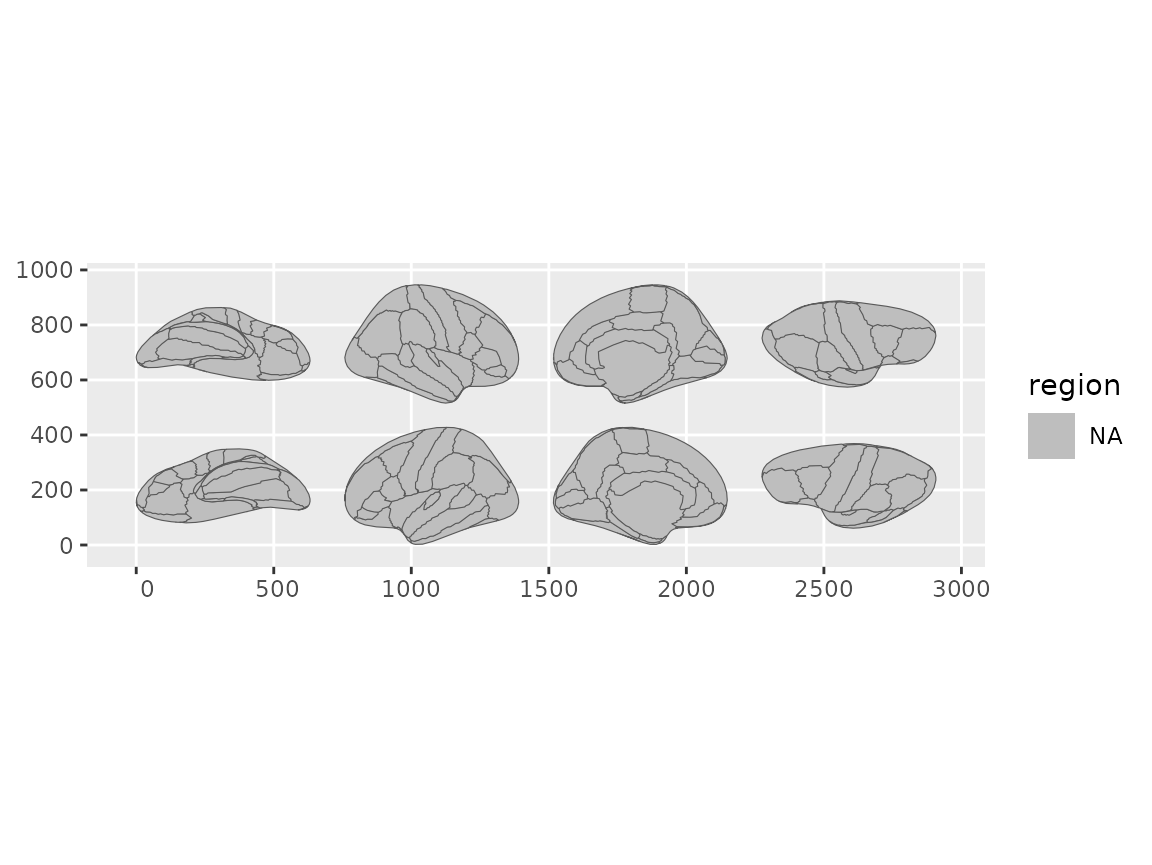
Brain views arranged using formula syntax in position_brain().
Or reorder views with a character vector:
ggplot() +
  geom_brain(
    atlas = dk(),
    position = position_brain(c(
      "right lateral",
      "right medial",
      "left lateral",
      "left medial"
    )),
    show.legend = FALSE
  )
Brain views arranged using a character vector to specify order.
See vignette("positioning-views") for the full set of
layout options, including grid layouts for subcortical and tract atlases
and per-view zoom.
Showing only certain hemispheres or views
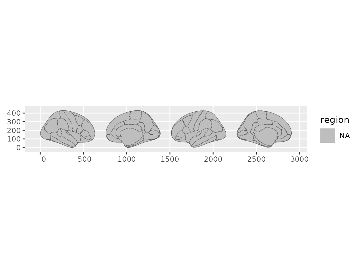
ggplot() +
  geom_brain(atlas = dk(), view = "lateral", show.legend = FALSE)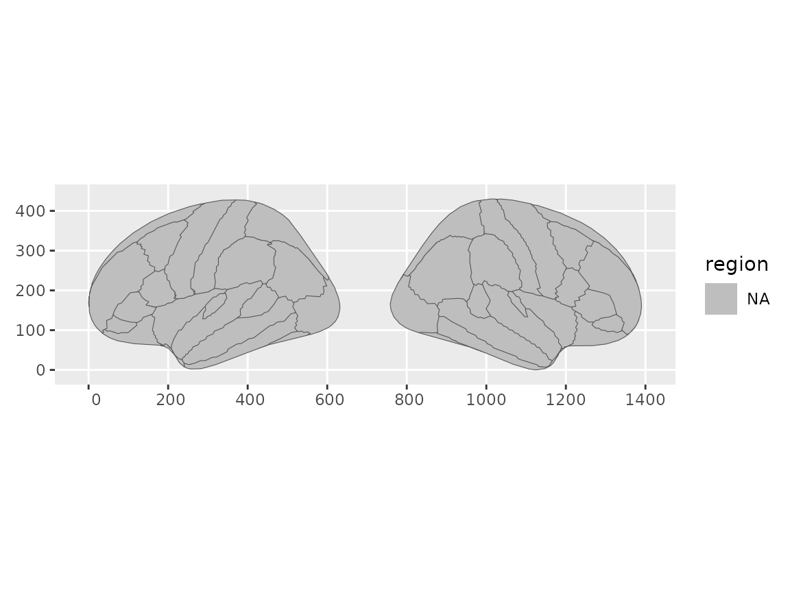
Brain plot showing only lateral views.
ggplot() +
  geom_brain(atlas = dk(), hemi = "left")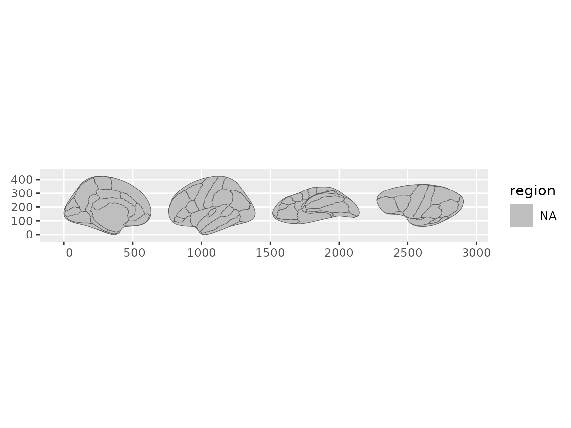
Brain plot showing only the left hemisphere.
For subcortical atlases, views are slice identifiers. Check what’s
available with ggseg.formats::atlas_views():
atlas_views(aseg())
#> [1] "axial_3"   "axial_4"   "axial_5"   "sagittal"  "axial_6"   "coronal_1"
#> [7] "coronal_2"
Plotting your own data
Create a data frame with at least one column that matches the atlas
(typically region or label). Pass it to
geom_brain() through the data argument and it
joins to the atlas automatically:
library(dplyr)
#>
#> Attaching package: 'dplyr'
#> The following objects are masked from 'package:stats':
#>
#>     filter, lag
#> The following objects are masked from 'package:base':
#>
#>     intersect, setdiff, setequal, union

some_data <- tibble(
  region = c(
    "transverse temporal",
    "insula",
    "precentral",
    "superior parietal"
  ),
  p = sample(seq(0, 0.5, 0.001), 4)
)

ggplot() +
  geom_brain(
    atlas = dk(),
    data = some_data,
    position = position_brain(hemi ~ view),
    aes(fill = p)
  ) +
  scale_fill_viridis_c(option = "cividis", direction = -1) +
  theme_void()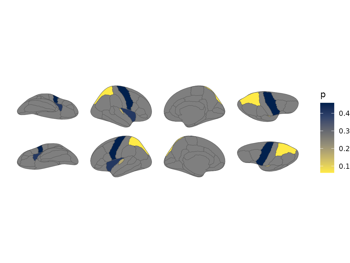
Brain plot coloured by external p-values using a viridis scale.
See vignette("external-data") for more on data
preparation and matching.
Faceting
ggplot2 faceting works as you’d expect. Group your data by the
faceting variable and geom_brain() replicates the full
atlas in each panel:
some_data <- tibble(
  region = rep(
    c(
      "transverse temporal",
      "insula",
      "precentral",
      "superior parietal"
    ),
    2
  ),
  p = sample(seq(0, 0.5, 0.001), 8),
  group = c(rep("A", 4), rep("B", 4))
)

ggplot() +
  geom_brain(
    atlas = dk(),
    data = group_by(some_data, group),
    position = position_brain(hemi ~ view),
    aes(fill = p)
  ) +
  facet_wrap(~group)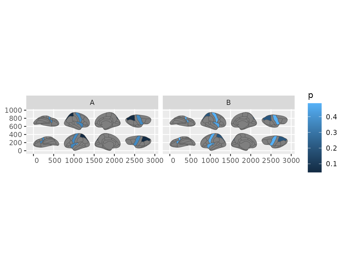
Brain plots faceted by group, each panel showing the full atlas.
Highlighting specific regions
To colour a few regions with their atlas colours, use two columns:
one for the join (region) and one for the fill
aesthetic:
data <- data.frame(
  region = atlas_regions(dk())[1:3],
  reg_col = atlas_labels(dk())[1:3]
)

palette <- atlas_palette(dk())[1:3]

ggplot() +
  geom_brain(atlas = dk(), data = data, aes(fill = reg_col)) +
  scale_fill_brain_manual(palette)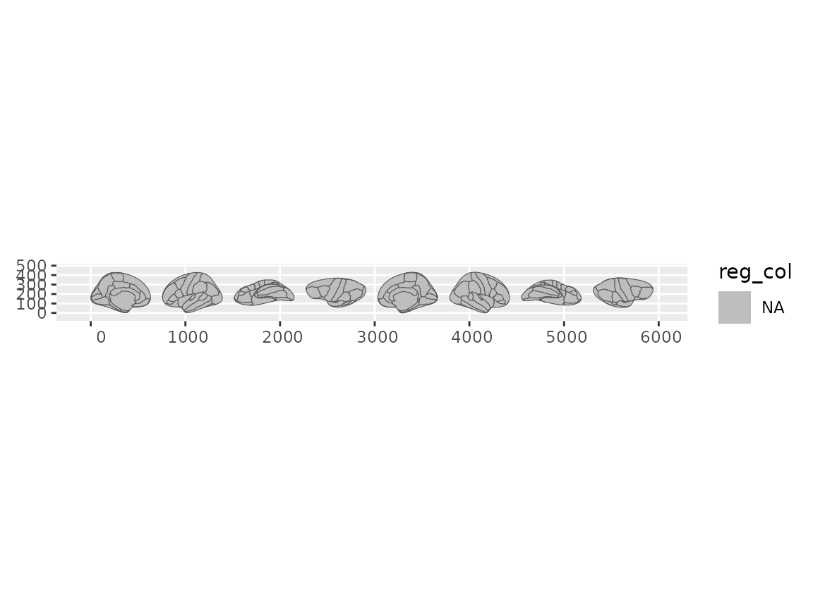
Highlighting selected regions using the atlas colour palette.
Scales and themes
Atlas colour palettes are applied automatically by
geom_brain(). For custom palettes, use
scale_fill_brain_manual().
Built-in themes strip axes and grids for cleaner figures:
ggplot() +
  geom_brain(atlas = dk()) +
  theme_brain()
Going further
For full control over the data before it reaches ggplot2 — adding
region labels, layering other sf geoms, or using geom_sf()
directly — see vignette("geom-sf").
Finding more atlases
ggseg ships with dk() (cortical), aseg()
(subcortical), suit() (cerebellar flamap), and
tracula() (white matter tracts). Many more are available
through the ggsegverse
r-universe:
install.packages("ggsegYeo2011", repos = "https://ggsegverse.r-universe.dev")