A brain atlas typically has several views – lateral and medial for
cortical atlases, or axial, coronal, and sagittal slices for subcortical
and tract atlases. position_brain() controls how those
views are arranged in the final plot.
The function works differently depending on the atlas type, so this vignette covers cortical and subcortical/tract atlases separately.
Cortical atlases
Cortical atlases like dk have two layout dimensions:
hemi (left or right) and view
(lateral, medial, etc.). The formula syntax mirrors
facet_grid() – left side is rows, right side is
columns:
ggplot() +
  geom_brain(
    atlas = dk(),
    position = position_brain(hemi ~ view),
    show.legend = FALSE
  ) +
  theme_void()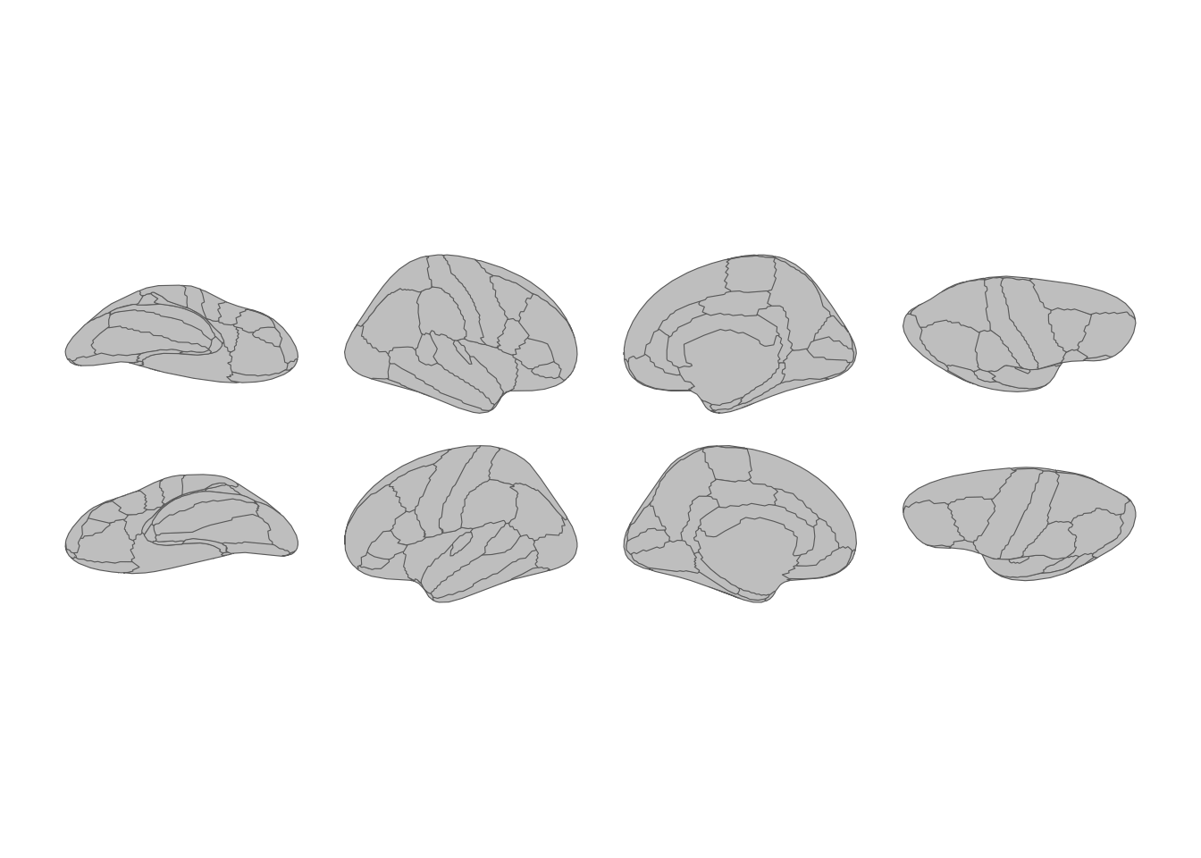
Cortical atlas with hemispheres as rows and views as columns.
Flip the formula to transpose the layout:
ggplot() +
  geom_brain(
    atlas = dk(),
    position = position_brain(view ~ hemi),
    show.legend = FALSE
  ) +
  theme_void()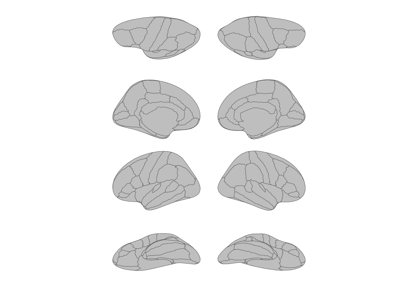
Transposed layout with views as rows and hemispheres as columns.
Stacking all views
Use . with + to collapse everything into a
single row or column. This is handy for compact figures:
ggplot() +
  geom_brain(
    atlas = dk(),
    position = position_brain(. ~ hemi + view),
    show.legend = FALSE
  ) +
  theme_void()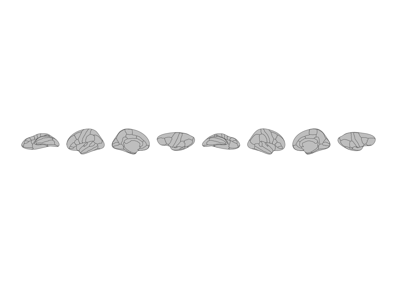
All brain views stacked in a single row.
ggplot() +
  geom_brain(
    atlas = dk(),
    position = position_brain(hemi + view ~ .),
    show.legend = FALSE
  ) +
  theme_void()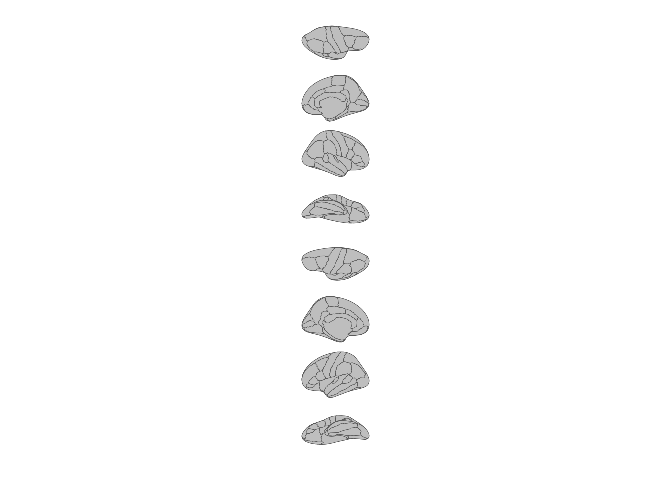
All brain views stacked in a single column.
Subcortical and tract atlases
Subcortical atlases like aseg and tract atlases like
tracula don’t have the hemisphere/view pairing that
cortical atlases do. Their views are individual slices
(e.g. "axial_3", "sagittal"). That opens up a
different set of positioning tools.
Horizontal and vertical
The simplest options. "horizontal" is the default:
ggplot() +
  geom_brain(
    atlas = aseg(),
    position = position_brain("horizontal"),
    show.legend = FALSE
  ) +
  theme_void()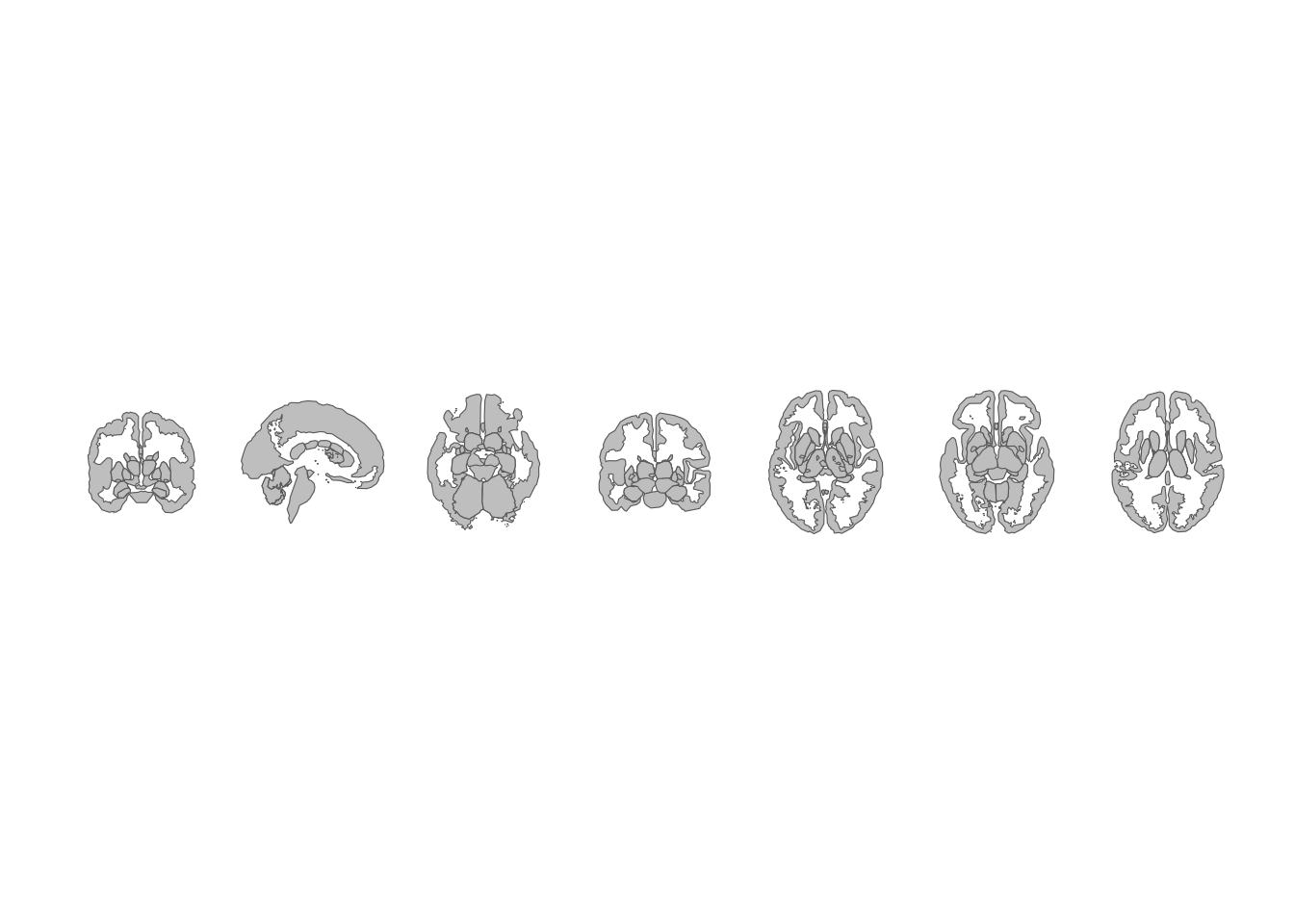
Subcortical atlas views arranged horizontally.
ggplot() +
  geom_brain(
    atlas = aseg(),
    position = position_brain("vertical"),
    show.legend = FALSE
  ) +
  theme_void()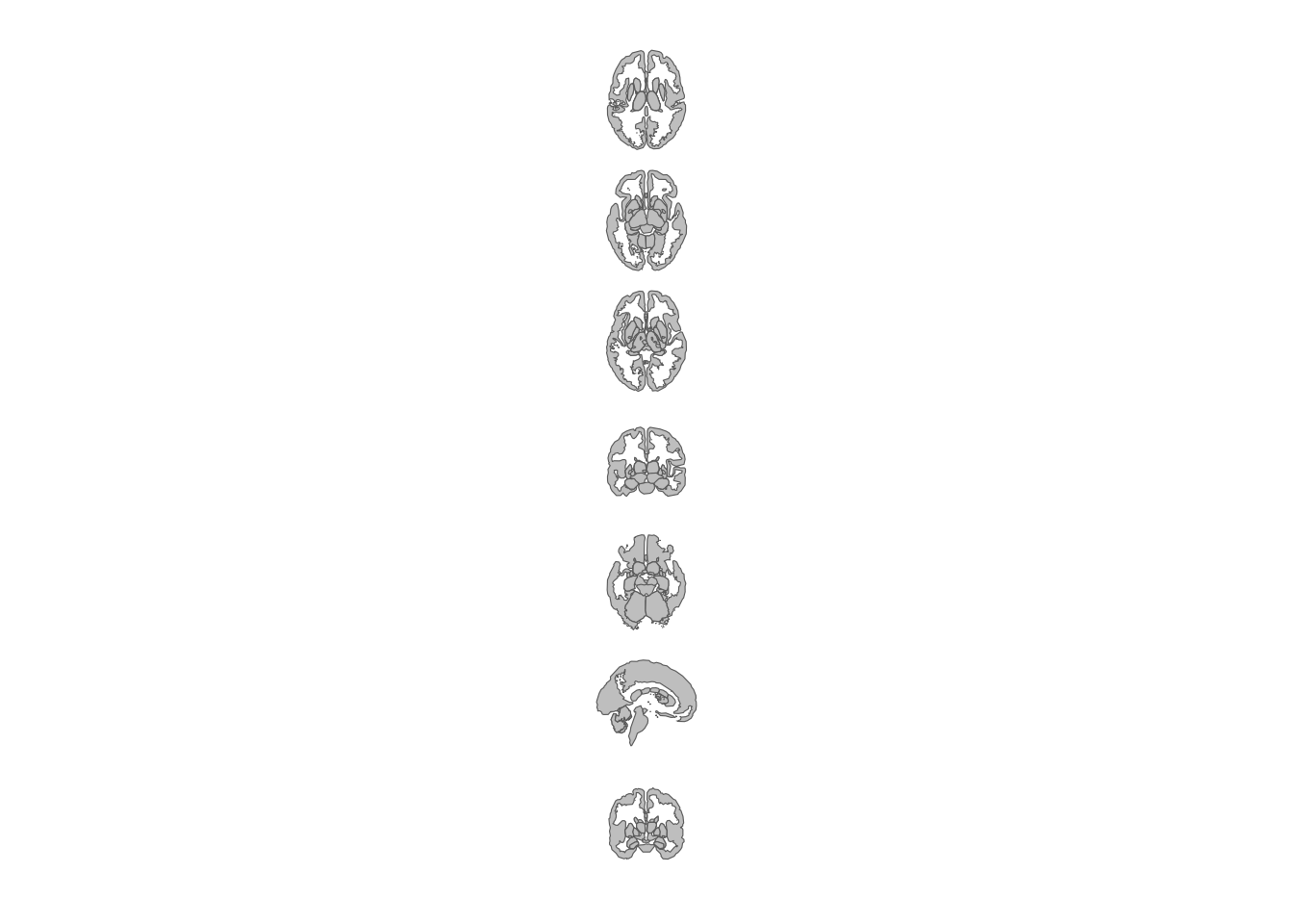
Subcortical atlas views arranged vertically.
Grid layouts
When you have many views, a grid keeps things readable. Specify
nrow, ncol, or both:
ggplot() +
  geom_brain(
    atlas = aseg(),
    position = position_brain(nrow = 2),
    show.legend = FALSE
  ) +
  theme_void()
Subcortical atlas views in a two-row grid.
ggplot() +
  geom_brain(
    atlas = aseg(),
    position = position_brain(ncol = 3),
    show.legend = FALSE
  ) +
  theme_void()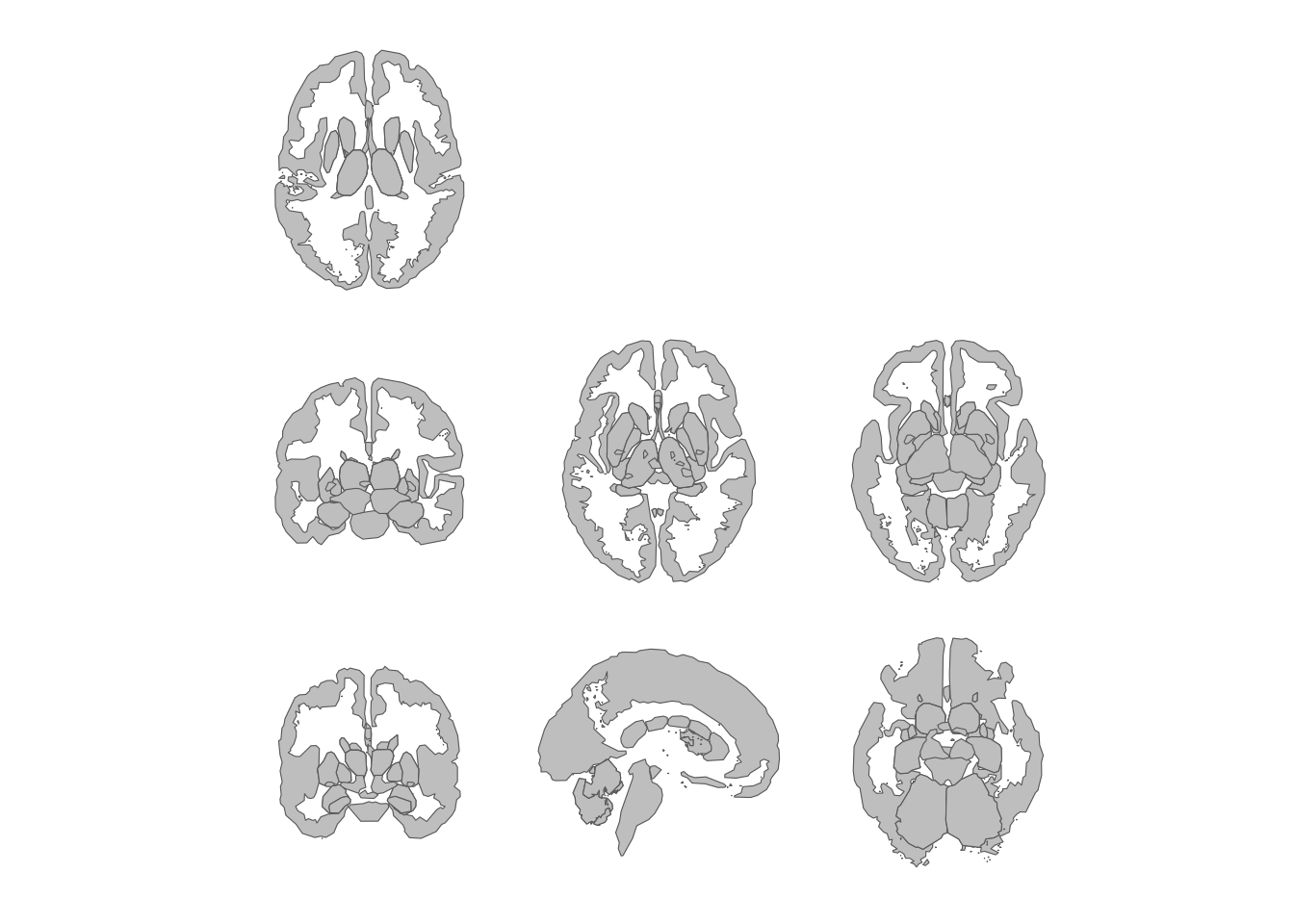
Subcortical atlas views in a three-column grid.
Picking specific views
The views parameter lets you select which views to
include and in what order. Check what’s available with
ggseg.formats::atlas_views():
ggseg.formats::atlas_views(aseg())
#> [1] "axial_3"   "axial_4"   "axial_5"   "sagittal"  "axial_6"   "coronal_1"
#> [7] "coronal_2"
ggplot() +
  geom_brain(
    atlas = aseg(),
    position = position_brain(
      views = c("sagittal", "axial_3", "coronal_3")
    ),
    show.legend = FALSE
  ) +
  theme_void()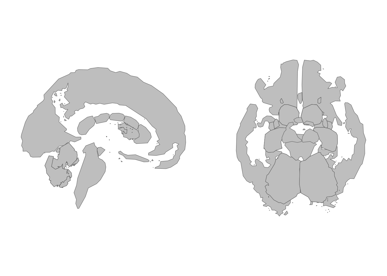
A subset of subcortical views selected by name.
Combine views with nrow or
ncol for a custom grid:
ggplot() +
  geom_brain(
    atlas = aseg(),
    position = position_brain(
      views = c("sagittal", "axial_3", "axial_5", "coronal_3"),
      nrow = 2
    ),
    show.legend = FALSE
  ) +
  theme_void()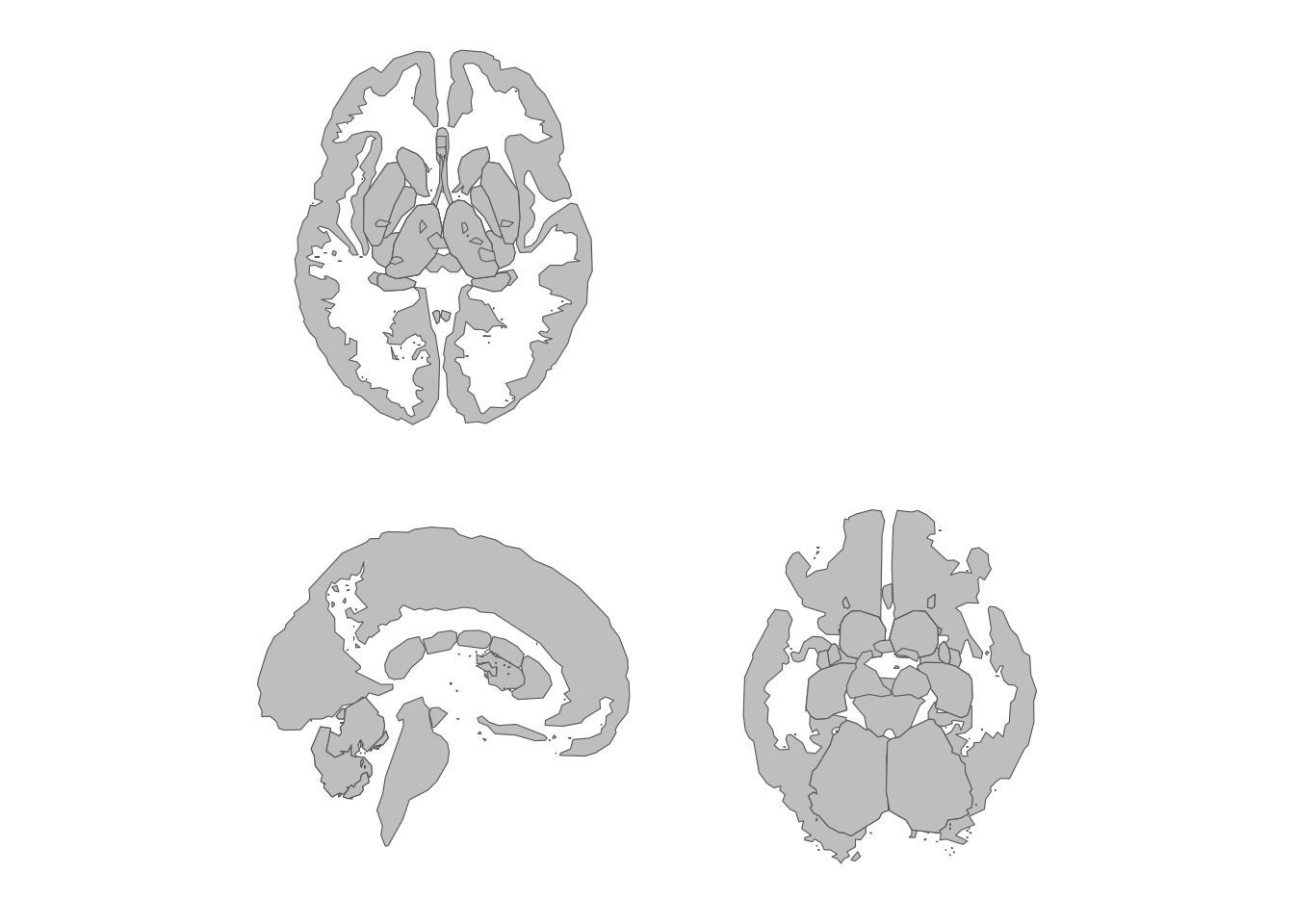
Custom two-row grid with selected subcortical views.
Grouping by slice type
The type ~ . formula groups views by their orientation –
all axial slices together, all coronal slices together, and so on. The
type is extracted from the view name (everything before the first
underscore):
ggplot() +
  geom_brain(
    atlas = aseg(),
    position = position_brain(type ~ .),
    show.legend = FALSE
  ) +
  theme_void()
Adding view labels
Use annotate_brain() to label each view with its name.
For cortical atlases the label combines hemisphere and view (e.g. “left
lateral”); for subcortical and tract atlases it uses the view name
directly.
Store the position_brain() specification in an object so
both layers share the same layout:
pos <- position_brain(hemi ~ view)
ggplot() +
  geom_brain(atlas = dk(), position = pos, show.legend = FALSE) +
  annotate_brain(atlas = dk(), position = pos) +
  theme_void()
Cortical atlas with view labels.
It works with any positioning — horizontal, vertical, grid, and formula layouts:
pos <- position_brain(nrow = 2)
ggplot() +
  geom_brain(atlas = aseg(), position = pos, show.legend = FALSE) +
  annotate_brain(atlas = aseg(), position = pos) +
  theme_void()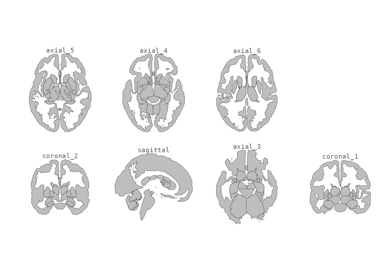
Subcortical atlas with view labels in a two-row grid.
Labels sit a little above each view by default
(padding = 0.05). Increase padding to push
them further out, and tune the text through standard
annotate() arguments:
ggplot() +
  geom_brain(atlas = dk(), show.legend = FALSE) +
  annotate_brain(
    atlas = dk(),
    padding = 0.08,
    size = 2.5,
    colour = "grey50",
    fontface = "italic"
  ) +
  theme_void()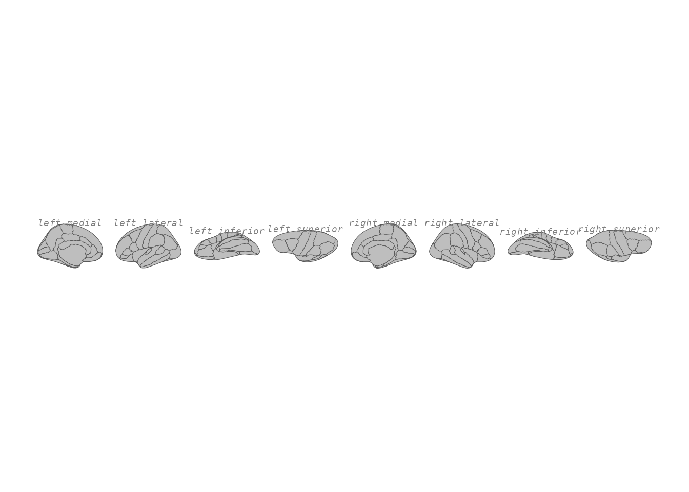
View labels with extra padding and custom styling.
Zooming in on regions of interest
For “focus” atlases – where only a few structures carry labels and
the rest of the brain is grey context –
position_brain(zoom = ...) crops each view onto the regions
of interest, so they fill the panel while the surrounding context
becomes a tidy grey frame. Every view keeps the same allotted cell.
Focus on the regions in your data
zoom = TRUE focuses on whatever regions your data
supplies values for (or, with no data, the atlas’s labelled
regions):
my_data <- data.frame(
  region = ggseg.formats::atlas_regions(aseg())[1:3],
  value = c(1, 2, 3)
)

ggplot() +
  geom_brain(
    atlas = aseg(),
    data = my_data,
    aes(fill = value),
    position = position_brain(zoom = TRUE)
  ) +
  scale_fill_viridis_c(na.value = "grey85") +
  theme_void()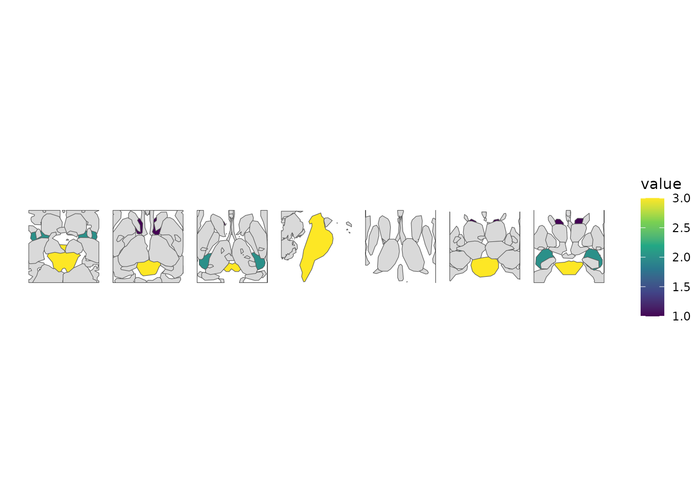
Each view zoomed onto the regions present in the supplied data.
Name the focus regions explicitly
Pass a character vector to choose exactly which regions each view zooms onto, independent of any data you plot:
focus <- c("Thalamus Proper", "Putamen", "Hippocampus")

ggplot() +
  geom_brain(
    atlas = aseg(),
    position = position_brain(zoom = focus),
    show.legend = FALSE
  ) +
  theme_void()
Zoom targeted at a named set of regions.
Control the margin with zoom_pad
zoom_pad sets how much breathing room to leave around
the focus regions, as a fraction of their size (5% by default). A
smaller value crops tighter; a larger value keeps more context in
frame:
ggplot() +
  geom_brain(
    atlas = aseg(),
    position = position_brain(zoom = focus, zoom_pad = 0.01),
    show.legend = FALSE
  ) +
  theme_void()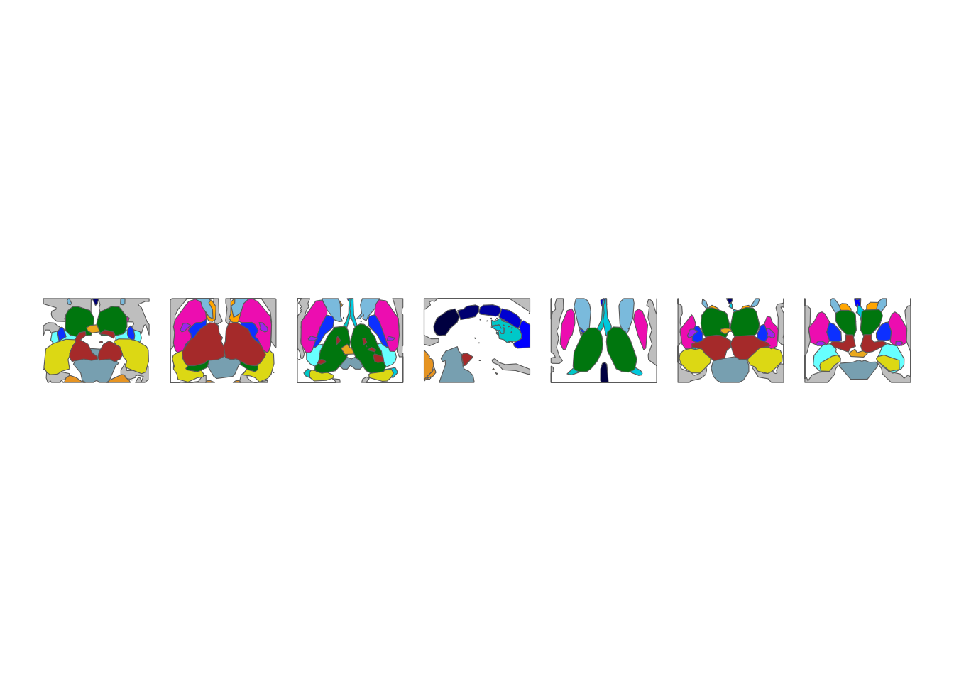
A tighter crop using a small zoom_pad.
ggplot() +
  geom_brain(
    atlas = aseg(),
    position = position_brain(zoom = focus, zoom_pad = 0.25),
    show.legend = FALSE
  ) +
  theme_void()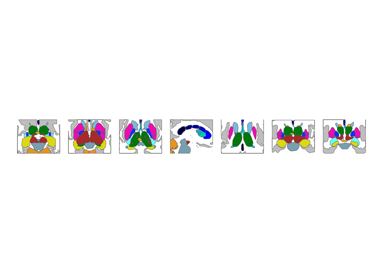
More surrounding context using a larger zoom_pad.
Dropping the grey context
Set context = FALSE to remove the unlabelled context
regions entirely. The remaining atlas regions are re-gathered into a
tighter layout:
ggplot() +
  geom_brain(atlas = aseg(), context = FALSE, show.legend = FALSE) +
  theme_void()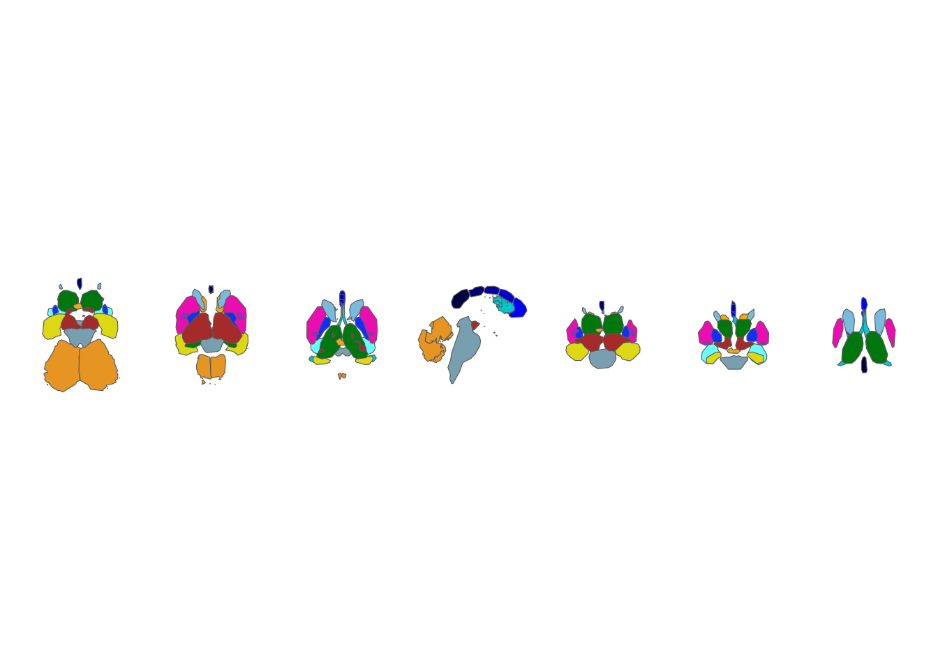
Subcortical atlas with the grey context regions removed.
The sf workflow
If you work with brain atlases as sf objects – for example to layer
geom_sf() text labels – reposition_brain()
rearranges the sf data using the same arguments shown here. See
vignette("geom-sf") for that workflow.