Neuroimaging analyses produce region-level results – cortical thickness, p-values, network assignments – that need to end up on a brain figure. ggseg stores brain atlas geometries as simple features and plots them as ggplot2 layers, so you get publication-ready brain figures with the same code you’d use for any other ggplot.
Mowinckel & Vidal-Piñeiro (2020). Visualization of Brain Statistics With R Packages ggseg and ggseg3d. Advances in Methods and Practices in Psychological Science.
Installation
Install from CRAN:
install.packages("ggseg")Or get the development version from the ggsegverse r-universe:
options(repos = c(
  ggsegverse = "https://ggsegverse.r-universe.dev",
  CRAN = "https://cloud.r-project.org"
))
install.packages("ggseg")
Quick start
Built-in atlases
ggseg ships with three atlases: dk (Desikan-Killiany cortical parcellation), aseg (automatic subcortical segmentation), and tracula (white matter tracts). plot() gives you a quick overview:
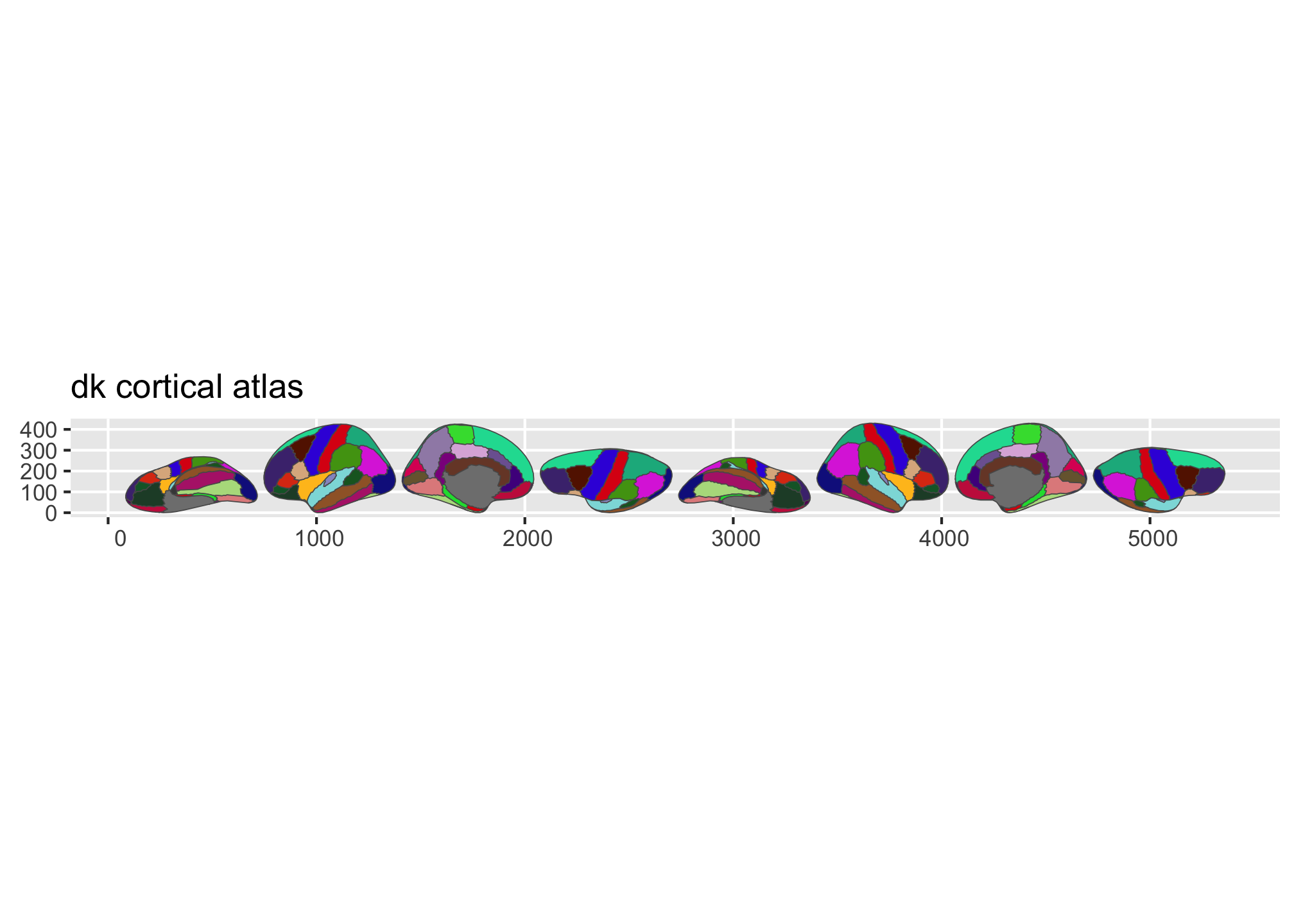
Figure 1: Overview of the dk and aseg built-in brain atlases.
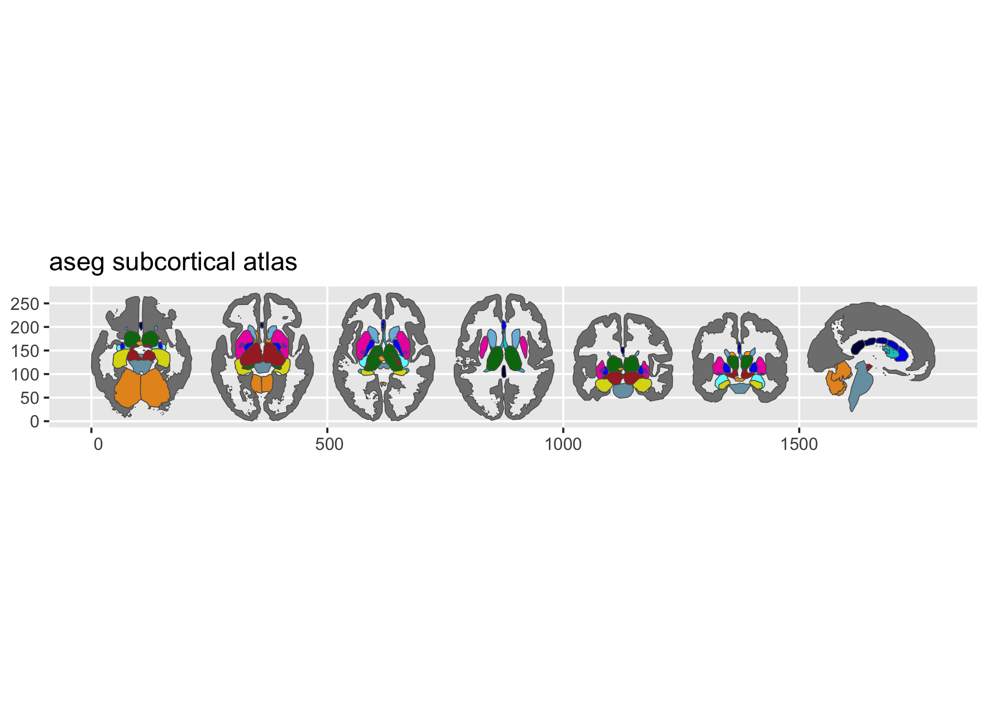
Figure 2: Overview of the dk and aseg built-in brain atlases.
Plotting your own data
Pass a data frame to ggplot() with a column that matches the atlas (typically region or label). geom_brain() handles the join:
library(dplyr)

some_data <- tibble(
  region = rep(
    c(
      "transverse temporal",
      "insula",
      "precentral",
      "superior parietal"
    ),
    2
  ),
  p = sample(seq(0, .5, .001), 8),
  groups = c(rep("g1", 4), rep("g2", 4))
)

ggplot(some_data) +
  geom_brain(
    atlas = dk(),
    position = position_brain(hemi ~ view),
    aes(fill = p)
  ) +
  facet_wrap(~groups) +
  scale_fill_viridis_c(option = "cividis", direction = -1) +
  theme_void()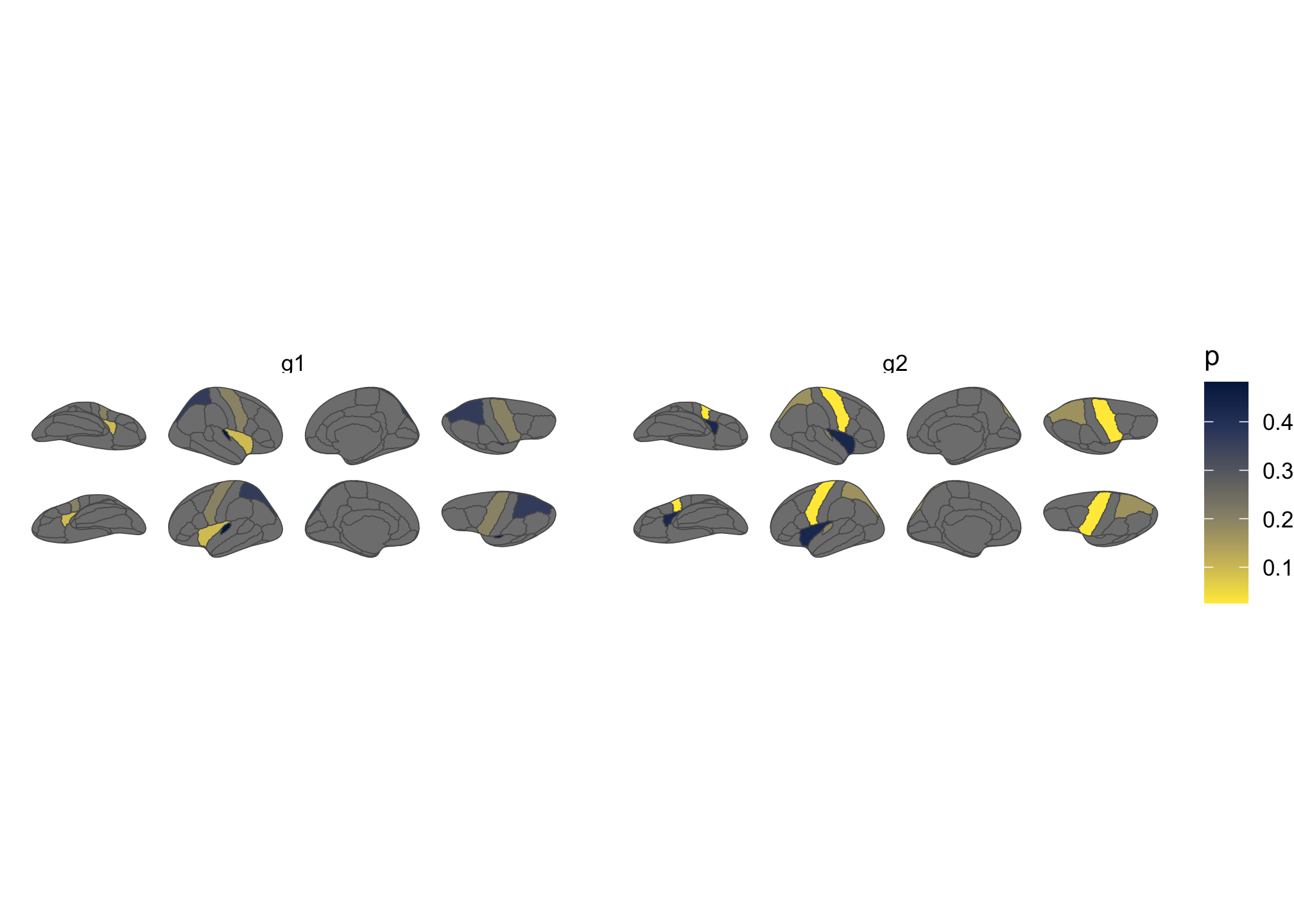
Figure 3: Brain plot coloured by external data, faceted by group.
More atlases
Many additional atlases are available through the ggsegverse r-universe:
install.packages("ggsegYeo2011", repos = "https://ggsegverse.r-universe.dev")Learn more
The package website has vignettes covering external data, view positioning, the geom_sf() workflow, and reading FreeSurfer stats files.